TensorFlow性能分析

In previous posts (here and here), I told you about how our team uses the Amazon SageMaker and Amazon s3 services to train our deep neural networks on large quantities of data.

在之前的文章( 此处和此处 )中，我告诉您我们的团队如何使用Amazon SageMaker和Amazon s3服务在大量数据上训练我们的深度神经网络。

In this blog, I would like to discuss how to profile the performance of a DNN training session running in TensorFlow. When speaking of the “performance” of a DNN training session, one may be referring to a number of different things. In the context of this blog, “performance” profiling will refer to analysis of the speed at which the training is performed (as measured, for example, by the training throughput or iterations per second), and the manner in which the session utilizes the system resources to achieve this speed. We will not be referring to the performance of the model being trained, often measured by the loss or metric evaluation on a test set. An additional measure of performance is the number of batches required until the training converges. This is also out of the scope of this blog.

在此博客中，我想讨论如何分析在TensorFlow中运行的DNN培训课程的性能。 当谈到DNN培训课程的“表现”时，可能是指许多不同的事物。 在本博客的上下文中，“性能”配置文件是指分析执行训练的速度(例如，通过训练吞吐量或每秒迭代次数来衡量)，以及会话利用该训练的方式的分析。系统资源实现这一速度。 我们不会指的是所训练模型的性能，通常是通过对测试集进行损失或度量评估来衡量的。 绩效的另一个衡量标准是培训收敛之前所需的批处理数量。 这也不在本博客的讨论范围之内。

In short, if you are trying to figure out why your training is running slowly, you have come to the right place. If you are searching for ways to improve the accuracy of your mnist model, or are searching for what optimizer settings to use to accelerate convergence, you have not.

简而言之，如果您试图弄清楚为什么培训运行缓慢，那么您来对地方了。 如果您正在寻找提高mnist模型准确性的方法，或者正在寻找用于加速收敛的优化器设置，那么您就没有了。

The examples we will review were written in TensorFlow and run in the cloud using the Amazon SageMaker service, but the discussion we will have is equally applicable to any other training environment.

我们将审阅的示例是使用TensorFlow编写的，并使用Amazon SageMaker服务在云中运行，但是我们将进行的讨论同样适用于任何其他培训环境。

序幕 (Prelude)

Any discussion on performance profiling your training requires that we be clear about what the goal is, or, what utility function we are trying to optimize. Your utility function will likely depend on a number of factors, including, the number of training instances at your disposal, the cost of those instances, the number of models you need to train, project scheduling constraints and more.

有关对您的培训进行性能分析的任何讨论都要求我们清楚目标是什么，或者我们正在尝试优化的实用程序功能。 您的实用程序功能可能取决于许多因素，包括可供您使用的训练实例数量，这些实例的成本，您需要训练的模型数量，项目进度约束等等。

In order to have a meaningful discussion, we will make some simplifying assumptions. Our goal will be to maximize the throughput of a training session, given a fixed training environment, without harming the quality of the resultant model, or increasing the number of training samples required for convergence.

为了进行有意义的讨论，我们将做一些简化的假设。 我们的目标是在固定的培训环境下 ， 最大程度地提高培训的吞吐量 ，而又不损害结果模型的质量，也不增加收敛所需的培训样本数量。

The goal, as stated, includes some ambiguities that we will promptly explain.

如前所述，目标包括一些歧义，我们将立即加以解释。

训练实例 (Training Instance)

Our first simplifying assumptions are that the training is being performed on a single instance/machine and that the instance type is fixed.

我们第一个简化的假设是，训练是在单个实例/机器上执行的，并且实例类型是固定的。

Naturally, different models perform differently on different types of machines. In an ideal situation, we would always be able to choose a machine that is optimal for the model being trained, that is, a machine on which all resources would be fully utilized. That way, we would avoid the cost of resources than are not being used. Unfortunately, in the real world, we are usually faced with a fixed number of instance types to choose from. For example, Amazon SageMaker offers a wide variety of instance types to choose from, that differ in the types and number of GPUs, the number of CPUs, the network properties, memory size and more. On the other hand, one does not have the ability to freely choose (based on the properties of their model) a machine with a specific number of CPUs, a specific GPU and specific network bandwidth.

自然地，不同的模型在不同类型的机器上表现不同。 在理想情况下，我们始终可以选择最适合所训练模型的机器，即可以充分利用所有资源的机器。 这样，我们将避免资源成本比没有使用的成本。 不幸的是，在现实世界中，我们通常面临固定数量的实例类型可供选择。 例如，Amazon SageMaker提供了多种实例类型供您选择，它们在GPU的类型和数量，CPU的数量，网络属性，内存大小等方面有所不同。 另一方面，没有能力(基于其模型的属性)自由选择具有特定数量的CPU，特定GPU和特定网络带宽的计算机。

In order to choose the most appropriate training instance, one must carefully weigh how well a model is suited to different training instances, versus considerations such as the cost and availability of those instances, as well as scheduling requirements. This requires a comprehensive analysis of the maximum achievable performance of training the model on each of the different instances types, as we describe in this post.

为了选择最合适的训练实例，必须仔细权衡模型对不同训练实例的适应程度，以及诸如这些实例的成本和可用性以及调度要求之类的考虑。 正如我们在这篇文章中所描述的，这需要对在每种不同实例类型上训练模型的最大可实现性能进行全面分析。

We will limit our discussion to instance types with a single GPU. Specifically, we will work on machines with an NVIDIA® V100 Tensor Core GPU. If you are using the Amazon SageMaker service for training, this is the ml.p3.2xlarge instance type.

我们将讨论仅限于具有单个GPU的实例类型。 具体来说，我们将在配备NVIDIA®V100 Tensor Core GPU的机器上工作。 如果您正在使用Amazon SageMaker服务进行培训，则这是ml.p3.2xlarge实例类型。

培训框架 (Training Framework)

There are many different libraries and frameworks available for training DNN models. As before, the training performance of a fixed model, fixed training algorithm and fixed HW, will vary across different SW solutions. As highlighted in the title of the post, our focus will be on the TensorFlow training environment. Even within this training environment, performance may depend on a number of factors such as the framework version, whether you choose a high level API, such as tf.estimator or tf.keras.model.fit, or implement a custom training loop, and the manner in which feed your training data into the training pipeline. Our assumptions in this post will be that the training will be performed in TensorFlow 2.2, using the tf.keras.model.fit() API, and that the data will be fed using the tf.dataset APIs.

有许多不同的库和框架可用于训练DNN模型。 和以前一样，固定模型，固定训练算法和固定硬件的训练性能在不同的软件解决方案之间会有所不同。 正如帖子标题中突出显示的那样，我们的重点将放在TensorFlow培训环境上。 即使在这种培训环境中，性能也可能取决于许多因素，例如框架版本，是否选择高级API(例如tf.estimator或tf.keras.model.fit)或实现自定义培训循环，以及将训练数据输入训练管道的方式。 我们在这篇文章中的假设是，训练将在TensorFlow 2.2中使用tf.keras.model.fit()API进行，并且数据将使用tf.dataset API进行馈送。

规则与约束 (Rules and Constraints)

Where there no constraints, speeding up the training throughput would be a piece of cake. For example, we could simply reduce the size of our model architecture and training would fly. Of course, this is likely to kill the ability of the training to converge and the resultant model predictions may be useless. Obviously, we must ensure that any actions we take to accelerate the training does not harm the quality of the resultant model.

在没有任何限制的情况下，加快训练吞吐量将是小菜一碟。 例如，我们可以简单地减小模型架构的大小，然后进行培训。 当然，这很可能会破坏训练的收敛能力，并且所得的模型预测可能是无用的。 显然，我们必须确保为加快培训速度而采取的任何措施都不会损害最终模型的质量。

For our discussion, we introduce an additional constraint, which is, that we do not want to impact the overall time required for training convergence, as measured by the overall number of training samples fed into the network until convergence. In other words, we make the simplifying assumption that our model requires a fixed number of training samples to converge and that the options we have to optimize will not change that fixed number. Based on that assumption, and given a fixed instance and SW environment, our goal is to optimize the overall amount of time (in seconds) that the training takes, or, alternatively, the training throughput, measured in the number of samples being processed by the training loop per second.

在我们的讨论中，我们引入了一个附加约束，即我们不想影响训练收敛所需的总时间，该时间由馈入网络直到收敛的训练样本的总数来衡量。 换句话说，我们做出简化的假设，即我们的模型需要固定数量的训练样本才能收敛，并且我们必须优化的选项不会更改该固定数量。 基于该假设，并在固定的实例和软件环境的情况下，我们的目标是优化训练所花费的总时间(以秒为单位)，或者以通过处理的样本数量衡量的训练吞吐量每秒训练循环。

We emphasize that this is an artificial constraint we introduce to simplify the discussion. There certainly may be situations where a change to the model architecture would increase the number of samples required for convergence, while reducing the overall time to convergence. For example, reducing the bit precision of some of the variables is likely to increase the throughput, but also might require more steps to converge. If the overall time to train is reduced, and the resultant model predicts just as well, then this would be a great optimization. Another important example is increasing the batch size. Increasing the training batch size is one of the basic ways to increase throughput. However, there are some models for which the training quality may be sensitive to the batch size. We make the simplifying assumption that such an impact is negligible and can be overcome by tuning other hyper-parameters (such as the learning rate).

我们强调这是我们引入的人为约束，旨在简化讨论。 当然，在某些情况下，对模型体系结构的更改将增加收敛所需的样本数量，同时减少收敛的总时间。 例如，降低某些变量的位精度可能会增加吞吐量，但也可能需要更多步骤才能收敛。 如果减少了训练的总时间，并且生成的模型也预测得很好，那么这将是一个很好的优化。 另一个重要的例子是增加批量大小。 增加训练批量大小是增加吞吐量的基本方法之一。 但是，有些模型的训练质量可能对批次大小敏感。 我们做出简化的假设，即这种影响可以忽略不计，并且可以通过调整其他超参数(例如学习率)来克服。

测量单位 (Measurement Units)

The units we will use to measure the throughput are the average number of samples processed by the training loop, per second. An, alternative, more common unit measurement for throughput is the average number of training iterations per second, steps per second, or batches per second. However, since this measurement is based on the chosen (global) batch size, it makes it hard to compare between runs that use different batch sizes.

我们将用来测量吞吐量的单位是训练循环每秒处理的平均样本数。 吞吐量的另一种更常见的单位度量是每秒训练迭代次数，每秒步数或每秒批处理的平均次数。 但是，由于此度量基于所选的(全局)批次大小，因此很难在使用不同批次大小的运行之间进行比较。

To extract this measurement, you can either rely on the logs that are printed by TensorFlow (at the end of every epoch), or implement the measurement on your own (e.g. with a custom TensorFlow callback).

要提取此度量，您可以依赖TensorFlow打印的日志(在每个时期的末尾)，也可以自己实施度量(例如，使用自定义的TensorFlow回调)。

优化策略 (Optimization Strategy)

Our main method for increasing training throughput is by increasing the utilization of the resources on our training instance. In theory, any under-utilized resource is a potential opportunity to increase throughput. However, practically speaking, once the GPU, the most expensive and important system resource, is fully utilized, and assuming we are satisfied with the performance of our GPU operations, we will consider our mission accomplished. We could, in theory, consider offloading some of the training to the CPU, but the performance gain would likely be negligible (if at all) — certainly not worth the headache. Under utilization could be a result of the pipeline not reaching its maximum capacity (e.g. all of the resources are under-utilized). In this case, increasing the throughput is fairly easy, (e.g. simply increase the batch size). If the pipeline is at maximum capacity, under-utilization of a system resource is typically the result of a bottleneck in the pipeline. For example, the GPU might be idle while it waits for training data to be prepared by the CPU. In such cases, we will attempt to increase the throughput by removing the bottleneck. For example, we might introduce parallelization between the CPU and GPU so that the GPU never has to wait for data.

我们增加训练吞吐量的主要方法是通过增加训练实例上资源的利用率。 从理论上讲，任何未充分利用的资源都是增加吞吐量的潜在机会。 但是，实际上，一旦最昂贵，最重要的系统资源GPU被充分利用，并且假设我们对GPU的运行性能感到满意，我们将认为我们的任务已经完成。 从理论上讲，我们可以考虑将一些培训工作转移给CPU，但是性能提升可能微不足道(如果有的话)，这当然不值得头疼。 利用率不足可能是管道未达到其最大容量的结果(例如，所有资源均未得到充分利用)。 在这种情况下，增加吞吐量相当容易(例如，简单地增加批次大小)。 如果管道处于最大容量，则系统资源的未充分利用通常是管道瓶颈的结果。 例如，GPU在等待CPU准备训练数据时可能处于空闲状态。 在这种情况下，我们将尝试通过消除瓶颈来提高吞吐量。 例如，我们可能会在CPU和GPU之间引入并行化，以便GPU永远不必等待数据。

The general strategy is to perform the following two steps recursively until we are satisfied with the throughput, or until the GPU is fully utilized:

一般的策略是递归执行以下两个步骤，直到我们对吞吐量感到满意或直到GPU被充分利用为止：

1. Profile the training performance to identify bottlenecks in the pipeline and under-utilized resources

1.概述培训绩效，以发现管道中的瓶颈和未充分利用的资源

2. Address bottlenecks and increase resource utilization

2.解决瓶颈并提高资源利用率

Note, that at any given time there may be more than one bottleneck in the pipeline. The CPU might be idle as it waits to receive data from the network, and the GPU might be idle as it waits for the CPU to prepare the data for training. Additionally, different bottlenecks might pop up at different stages of the training. For example, the GPU might be fully utilized but idle only during iterations when we save a checkpoint. Such bottlenecks, even if only periodic, could still potentially have a significant impact on the average throughput and should be addressed.

请注意，在任何给定时间，管道中可能存在多个瓶颈。 CPU在等待从网络接收数据时可能处于空闲状态，而GPU在等待CPU准备数据进行训练时可能处于空闲状态。 此外，在培训的不同阶段可能会弹出不同的瓶颈。 例如，当我们保存检查点时，GPU可能会被充分利用，但仅在迭代期间处于空闲状态。 这种瓶颈，即使只是周期性的，仍可能对平均吞吐量产生重大影响，应予以解决。

为什么性能分析很重要？ (Why is Performance Profiling Important?)

This should be abundantly clear by now, but sometimes the obvious requires stating. All too often, I have encountered developers who are perfectly content with 40% GPU utilization. It makes me want to scream. The GPU is (usually) the most expensive resource you are using; if you are happy with any less than 90% utilization, you are wasting your (your company’s) money. Not to mention that you could probably be delivering your product much sooner.

到现在为止，这应该已经很清楚了，但有时需要说明。 我经常遇到开发人员，他们对40％的GPU利用率非常满意。 这让我想尖叫。 GPU(通常)是您使用的最昂贵的资源。 如果您对利用率低于90％感到满意，那就是在浪费您(公司的)钱。 更不用说您可能会更快地交付产品。

It’s all about the money. Training resources are expensive, and if you are not maximizing their utilization, you are committing a crime against humanity.

这都是关于金钱的。 培训资源是昂贵的，并且如果您没有最大程度地利用它们，那么您将犯有危害人类罪。

I hope you are convinced of the importance of profiling your training performance and maximizing resource utilization. In the next section we will review some of the potential bottlenecks in a typical training pipeline. We will then survey some of the tools at your disposal for identifying these bottlenecks.

我希望您深信分析培训成绩并最大限度地利用资源的重要性。 在下一部分中，我们将回顾典型培训渠道中的一些潜在瓶颈。 然后，我们将调查您可以使用的一些工具来识别这些瓶颈。

培训管道和潜在瓶颈 (The Training Pipeline and Potential Bottlenecks)

In order to facilitate the discussion on the possible bottlenecks within a training session, we present the following diagram of a typical training pipeline. The training is broken down into eight steps, each of which can potentially impede the training flow. Note that while in this diagram training is performed on multiple GPUs, in this post, as mentioned above, we will assume that there is just one GPU.

为了促进对培训课程中可能出现的瓶颈的讨论，我们提供了以下典型培训流水图。 培训分为八个步骤，每个步骤都可能会阻碍培训流程。 请注意，虽然在该图中训练是在多个GPU上进行的，但是如上所述，在本文​​中，我们将假设只有一个GPU。

原始数据输入 (Raw Data Input)

Unless you are auto-generating your training data, you are likely loading it from storage. This might be from local disk or it might be over the network, from a remote storage location. In either case, you are using system resources that could potentially block the pipeline. If the amount of raw data per training sample is particularly large, if your IO interface has high latency, or if the network bandwidth of your training instance is low, you may find your CPU sitting idly as it waits for the raw data to come in. A classic example of this is if you train with Amazon SageMaker using “filemode”. In “filemode” all of the training data is downloaded to local disk before the training even starts. If you have a lot of data, you could be waiting a while. The alternative Amazon Sagemaker option is to use “pipemode”. This allows you to stream data directly from s3 into your input data pipeline, thus avoiding the huge bottleneck to training startup. But even in the case of “pipemode” you can easily run up on resource limitations. For example, if your instance type supports network IO of up to 10 Gigabits per second, and each sample requires 100 Megabits of raw data, you will have an upper limit of 100 training samples per second, no matter how fast your GPU is. The way to overcome such issues is to reduce your raw data, compress some of the data or to choose an instance type with a higher network IO bandwidth.

除非您自动生成训练数据，否则很可能会从存储中加载它。 这可能来自本地磁盘，也可能来自网络，来自远程存储位置。 无论哪种情况，您都在使用可能会阻塞管道的系统资源。 如果每个训练样本的原始数据量特别大，IO接口具有较高的延迟或训练实例的网络带宽较低，则您可能会发现CPU闲置，因为它等待原始数据进入一个典型的例子是，如果您使用“ filemode”与Amazon SageMaker一起训练。 在“文件模式”下，所有培训数据甚至在培训开始之前都已下载到本地磁盘。 如果您有大量数据，则可能需要等待一段时间。 备选的Amazon Sagemaker选项是使用“ pipemode”。 这使您可以将数据直接从s3流传输到输入数据管道中，从而避免了培训启动的巨大瓶颈。 但是，即使在“管道模式”的情况下，您也可以轻松满足资源限制。 例如，如果您的实例类型支持每秒高达10 Gigabit的网络IO，并且每个样本都需要100 MB的原始数据，则无论您的GPU速度有多快，每秒都有100个训练样本的上限。 解决此类问题的方法是减少原始数据，压缩某些数据或选择具有更高网络IO带宽的实例类型。

In the example we gave, the limitation came from the network IO bandwidth of the instance, but it could also come from a bandwidth on the amount of data that you can pull from s3, or from somewhere else along the line. (Side note: if you are pulling data from s3 without using pipe mode, make sure to choose an instance type with Elastic Network Adapter enabled.)

在我们给出的示例中，限制来自实例的网络IO带宽，但也可能来自可从s3或沿线其他地方提取的数据量的带宽。 (附带说明：如果要在不使用管道模式的情况下从s3提取数据，请确保选择启用了Elastic Network Adapter的实例类型。)

数据预处理 (Data Preprocessing)

The next step in the training pipeline is the data pre-processing. In this stage, typically performed on the CPU, the raw data is prepared for entry to the training loop. This might include applying augmentations to input data, inserting masking elements, batching, filtering and more. The tensorflow.dataset functions include built-in functionality for parallelizing the processing operations within the CPU (e.g. the num_parallel_calls argument in the tf.dataset.map routine), and also for running the CPU in parallel with the GPU (e.g. tf.dataset.prefetch). However, if you are running heavy, or memory intensive computation in this stage, you might still find yourself with your GPU idle as it waits for data input.

训练流程的下一步是数据预处理。 在此阶段(通常在CPU上执行)，准备原始数据以输入训练循环。 这可能包括对输入数据进行扩充，插入掩蔽元素，批处理，过滤等。 tensorflow.dataset函数包括内置功能，用于并行化CPU中的处理操作(例如tf.dataset.map例程中的num_parallel_calls参数)，还用于与GPU并行运行CPU(例如tf.dataset)。预取)。 但是，如果在此阶段运行繁重的计算或占用大量内存的计算，则在等待数据输入时，GPU可能仍处于空闲状态。

CPU到GPU的数据传输 (CPU to GPU Data Transfer)

In most cases, your CPU and GPU use different memory, and the training samples need to be copied from CPU memory to GPU memory before the training loop can run. This too could potentially result in a bottleneck, depending on the size of your data samples and the interface bandwidth. One thing you should consider, wherever possible, is to hold off on casting to higher bit representation (tf.cast()) or decompressing bit masks (tf.one_hot), until after the data is copied to GPU memory.

在大多数情况下，您的CPU和GPU使用不同的内存，并且需要在训练循环运行之前将训练样本从CPU内存复制到GPU内存。 这也可能导致瓶颈，具体取决于数据样本的大小和接口带宽。 您应该考虑的一件事是，在将数据复制到GPU内存之前，推迟转换为更高的位表示形式(tf.cast())或解压缩位掩码(tf.one_hot)。

GPU后退 (GPU Forward Backward)

The heart of the training pipeline is the forward and backward pipeline. This step is performed on the GPU. Being that the GPU is the most expensive resource, we want the GPU to constantly be active and at peak performance. In most cases, the average throughput, in number of samples trained per second, increases as we increase the batch size, so we will try to increase the batch size up to the GPU’s memory capacity.

培训管道的核心是前进和后退管道。 此步骤在GPU上执行。 由于GPU是最昂贵的资源，因此我们希望GPU始终保持活动状态并达到最佳性能。 在大多数情况下，平均吞吐量(以每秒训练的样本数为单位)随着批量大小的增加而增加，因此，我们将尝试将批量大小增加到GPU的内存容量。

Obviously, the throughput of this step is a function of your model architecture and your loss function. There are quite a number of common methods for reducing the computation. Here is a very small sample of them:

显然，此步骤的吞吐量取决于模型架构和损失函数。 有很多减少计算的常用方法。 这是其中的一小部分样本：

· prefer conv layers over dense layers

·更喜欢转化层而不是致密层

· replace large convolutions with a series of smaller ones with the same receptive field

·用一系列具有相同接收场的较小卷积代替大型卷积

· use low precision or mixed precision variable types

·使用低精度或混合精度变量类型

· consider using TensorFlow native functions instead of tf.py_func

·考虑使用TensorFlow本机函数代替tf.py_func

· prefer tf.where over tf.cond

·更喜欢tf.where比tf.cond

· research how your model and layer settings, such as memory layout (channels first or last), and memory alignment (layer input and output size, number of channels, shapes of convolutional filters, etc) impact your GPU performance and design your model accordingly

·研究模型和图层设置(例如内存布局(第一个或最后一个通道)以及内存对齐方式(图层输入和输出大小，通道数，卷积滤波器的形状等))如何影响GPU性能并相应地设计模型

· customize the graph optimization

·自定义图形优化

渐变共享 (Gradient Sharing)

This step is only performed when training running distributed training on multiple GPUs, either on a single training instance or on multiple instances. We leave the discussion on distributed training for a future post, but will note that this step can also potentially introduce a bottleneck. During distributed training, each GPU must collect the gradients from all other GPUs. Depending on the distribution strategy, the number and size of the gradients, and the bandwidth of the communication channel between GPUs, a GPU may find itself idle while it collects the gradients. To solve such issues, one might reduce the bit precision of the gradients, tune the communication channel or consider other distribution strategies.

仅当训练在单个训练实例或多个实例上的多个GPU上运行分布式训练时，才执行此步骤。 我们将对分布式培训的讨论留在以后的文章中，但要注意的是，这一步骤也可能会带来瓶颈。 在分布式训练期间，每个GPU必须从所有其他GPU收集梯度。 根据分布策略，梯度的数量和大小以及GPU之间的通信通道的带宽，GPU在收集梯度时可能会发现自己处于空闲状态。 为了解决这些问题，可能会降低梯度的位精度，调整通信通道或考虑其他分配策略。

GPU到CPU的数据传输 (GPU to CPU Data Transfer)

During training, the GPU will return data to the CPU. Typically, this will include the loss and metric results, but may, periodically, also include more memory intensive output tensors or model weights. As before, this data transfer can potentially introduce a bottleneck at certain phases of the training, depending on the size of the data and the interface bandwidth.

在训练期间，GPU将数据返回给CPU。 通常，这将包括损失和度量结果，但可能会定期包含更多内存密集型输出张量或模型权重。 与以前一样，此数据传输可能会在训练的某些阶段引入瓶颈，具体取决于数据的大小和接口带宽。

模型输出处理 (Model Output Processing)

The CPU might perform some processing on the output data received from the GPU. This processing typically occurs within TensorFlow callbacks. These can be used to evaluate tensors, create image summaries, collect statistics, update the learning rate and more. There are different ways in which this could reduce the training throughput:

CPU可能会对从GPU接收到的输出数据执行某些处理。 此处理通常在TensorFlow回调中进行 。 这些可用于评估张量，创建图像摘要，收集统计信息，更新学习率等等。 有多种方法可以减少训练吞吐量：

· If the processing is computation or memory intensive, this may become a performance bottleneck. If the processing is independent of the model GPU state, you might want to try running in a separate (non-blocking) thread.

·如果处理过程需要计算或占用大量内存，则可能会成为性能瓶颈。 如果处理与模型GPU状态无关，则可能要尝试在单独的(非阻塞)线程中运行。

· Running a large number of callbacks could also bottleneck the pipeline. You might want to consider combining them into a small number.

·运行大量的回调也可能成为管道的瓶颈。 您可能需要考虑将它们合并为少量。

· If your callbacks are processing output on every iteration, you are also likely to be slowing down the throughput. Consider reducing the frequency of the processing, or adding the processing to the GPU model graph (e.g. using custom TensorFlow metrics).

·如果您的回调在每次迭代中都处理输出，则还可能会降低吞吐量。 考虑减少处理的频率，或将处理添加到GPU模型图(例如，使用自定义TensorFlow指标 )。

CPU到存储 (CPU to Storage)

During the training, the CPU might periodically transfer event files, log files or model checkpoints to storage. As before, a large quantity of data combined with a limited IO bandwidth, could potentially lead to latency in the training pipeline. Even if we are careful to make the data transfer non-blocking (e.g. using dedicated CPU threads), you might be using network input and output channels that share the same limited bandwidth (as on Amazon SageMaker instances). In this case, the amount of raw training data being fed on the network input, could drop.

在培训期间，CPU可能会定期将事件文件，日志文件或模型检查点传输到存储中。 和以前一样，大量数据与有限的IO带宽结合在一起，有可能导致训练流水线中出现延迟。 即使我们小心地使数据传输无阻塞(例如，使用专用的CPU线程)，您可能仍在使用共享相同有限带宽的网络输入和输出通道(例如在Amazon SageMaker实例上)。 在这种情况下，通过网络输入提供的原始训练数据量可能会减少。

One way this could happen is if we collect all of our TensorFlow summaries in a single event file which grows and grows during the course of the training. Each time the event file is uploaded to s3, the amount of data passing on the network increases. When the file becomes very large, the data upload can interfere with the training.

发生这种情况的一种方法是，如果我们将所有TensorFlow摘要收集在一个事件文件中，该文件在训练过程中会不断增长。 每次将事件文件上载到s3时，网络上传递的数据量都会增加。 当文件变得很大时，数据上传会干扰训练。

绩效分析工具 (Performance Analysis Tools)

Now that we have an understanding of some of the bottlenecks we might face in a training pipeline, let’s review some of the tools and techniques at your disposal for identifying and analyzing them.

既然我们已经了解了培训渠道中可能遇到的一些瓶颈，那么让我们回顾一下您可以使用的一些工具和技术，以识别和分析它们。

实例指标 (Instance Metrics)

A good place to start is to assess how the resources of the training instance are being utilized. In Amazon SageMaker these are provided as “Instance Metrics” which are displayed in the “Monitor” section of the training job page, as well as in Amazon SageMaker Studio. Here is an example of how this appears on the training job page:

一个很好的起点是评估培训实例的资源是如何被利用的。 在Amazon SageMaker中，这些作为“实例指标”提供，显示在培训作业页面的“监视器”部分以及Amazon SageMaker Studio中。 这是在培训作业页面上如何显示的示例：

Instance Metrics (from AWS console)

实例指标(从AWS控制台)

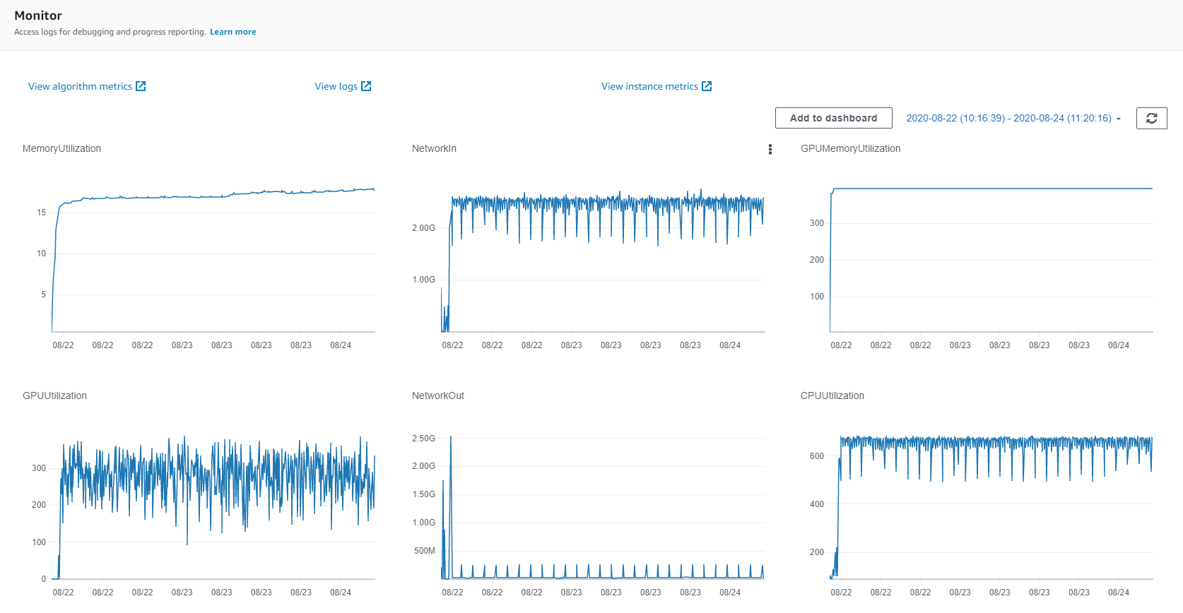
The Instance Metrics include graphs of the memory utilization, CPU utilization, network in, network out, GPU memory utilization, GPU utilization, and disk utilization, where measurements are displayed at five minute intervals. You can use this to make sure things are running as expected and to get a high level indication of what can be improved. (We refer to this as “high level” because of the relatively infrequent measurements.) For example, you can verify that you are, in fact, running on the GPU, and assess how well you are using it. In addition, you can identify anomalies in the different metrics such as:

实例指标包括内存利用率，CPU利用率，网络输入，网络输出，GPU内存利用率，GPU利用率和磁盘利用率的图形，其中每隔五分钟显示一次测量。 您可以使用它来确保一切按预期运行，并获得可以改进的高级指示。 (由于测量的频率相对较低，因此我们将其称为“高级别”。)例如，您可以验证您实际上是否在GPU上运行，并评估使用效果如何。 此外，您可以识别不同指标中的异常，例如：

· dips in the CPU/GPU utilization which could indicate a bottleneck

·CPU / GPU利用率下降可能表明存在瓶颈

· rising CPU memory which could indicate a memory leak

·CPU内存增加，这可能表明内存泄漏

· a choppy network-in could indicate an issue with how we are pulling data from s3

·断断续续的网络连接可能表明我们如何从s3中提取数据存在问题

· if the network-in is at maximum capacity (when compared to the training instance properties) this could indicate a bottleneck on the input pipeline

·如果网络输入最大容量(与训练实例属性相比)，则可能表明输入管道上存在瓶颈

· a rising network-out could indicate that we are uploading a single file that keeps growing instead of uploading small files

·网络中断上升可能表明我们正在上传一个不断增长的文件，而不是上传小文件

· a delay in GPU start time could indicate a lengthy model compilation period

·GPU启动时间的延迟可能表明模型编译期很长

One thing worth noting is that the default behavior of TensorFlow, is to take up all of the GPU memory. So don’t be overly alarmed (or happy) that the GPU memory utilization shows 100%. To configure TesorFlow to use only the memory it actually needs, you need to apply the lines of code below.

值得注意的是TensorFlow的默认行为是占用所有GPU内存。 因此，不要过度警惕(或高兴)GPU内存利用率显示为100％。 要将TesorFlow配置为仅使用其实际需要的内存，您需要应用以下代码行。

gpus = tf.config.experimental.list_physical_devices('GPU')for gpu in gpus:
    tf.config.experimental.set_memory_growth(gpu, True)

Pressing on the “View Instance Metrics” link will take you to the CloudWatch Management Console, where you can play around a bit with the measurements and graphs. For example, you can zoom in to specific intervals of the training, decrease the measurement intervals (to one minute), and display multiple metrics on a single graph.

按下“查看实例指标”链接将带您到CloudWatch管理控制台，您可以在其中玩弄一些度量和图表。 例如，您可以放大训练的特定间隔，将测量间隔减小(至一分钟)，并在单个图形上显示多个指标。

SageMaker allows you to include your own, custom, metrics in this window as well. These are referred to as “Algorithm Metrics”. For details, see the SageMaker documentation. For example, you can define the training throughput as a metric and have it displayed in this window as well.

SageMaker还允许您在此窗口中包括自己的自定义指标。 这些被称为“算法指标”。 有关详细信息，请参见SageMaker文档 。 例如，您可以将训练吞吐量定义为度量标准，并将其显示在此窗口中。

This method of performance analysis leaves much to be desired. Aside from the infrequency of the measurements, we receive little information regarding which parts of code require improvement. An under utilized GPU could stem from a low batch size or from a bottleneck. A highly utilized GPU may be a result of an inefficient loss function. Getting more information will require some heavier artillery.

这种性能分析方法还有很多不足之处。 除了测量频率不高外，我们几乎没有收到有关哪些部分代码需要改进的信息。 未充分利用的GPU可能是由于批量大小低或瓶颈引起的。 利用率高的GPU可能是低效损失函数的结果。 获取更多信息将需要一些重炮。

If you are running on your own training instance and not within the SageMaker service, you will need to collect the “instance metrics” yourself using, common, off-the-shelf system profilers. In a linux environment you can use command line tools such as nmon, perf, strace, top and iotop. If you are using an NVIDIA® GPU you can use nvidia-smi (with the -l flag).

如果您是在自己的训练实例上运行，而不是在SageMaker服务中运行，则需要使用通用的现成系统概要分析器自行收集“实例度量”。 在Linux环境中，您可以使用命令行工具，例如nmon，perf，strace，top和iotop。 如果您使用的是NVIDIA®GPU，则可以使用nvidia-smi(带有-l标志)。

性能分析器 (Performance Profilers)

To get a more in depth picture of how the different stages of your training session are performing, you should use a performance profiler. Different profilers are available for different development frameworks. TenorFlow offers the TensorFlow Profiler for profiling tf models. Your first encounter with a performance profiler can be a bit intimidating. There are often multiple graphs, that might appear overloaded and seem, at first, confusing. It is not always immediately clear how to interpret the wealth of data that is reported. But once you get the hang of it, profilers can be very useful in evaluating resource utilization, identifying bottlenecks and improving model performance.

要更深入地了解培训课程的不同阶段的执行情况，应使用性能分析器。 不同的探查器可用于不同的开发框架。 TenorFlow提供了用于分析tf模型的TensorFlow Profiler 。 您第一次遇到性能分析器可能会有些吓人。 通常有多个图，这些图可能看起来超载，乍一看似乎令人困惑。 并不总是立即清楚如何解释所报告的大量数据。 但是，一旦掌握了它，分析器就可以非常有用地评估资源利用率，识别瓶颈并提高模型性能。

TensorFlow Profiler

TensorFlow分析器

Check out the TensorFlow Profiler Guide and the TensorBoard Profiler Tutorialc for instructions on how to use the profiler. When training with tf.keras.model.fit(), the easiest way to integrate profiling is by using the TensorBoard Keras Callback as follows:

查看TensorFlow Profiler指南和TensorBoard Profiler Tutorialc，以获取有关如何使用Profiler的说明。 使用tf.keras.model.fit()进行训练时，最简单的集成分析方法是使用TensorBoard Keras回调 ，如下所示：

tbc = tf.keras.callbacks.TensorBoard(log_dir='/tmp/tb',       
                                     profile_batch='20, 24')

This will capture statistics on iterations 20 to 24 and save them to a file that can be opened and analyzed in TensorBoard. (The size of the interval impacts the amount of data captured.)

这将捕获有关迭代20至24的统计信息，并将其保存到可以在TensorBoard中打开和分析的文件中。 (时间间隔的大小会影响捕获的数据量。)

Note that the TensorFlow Profiler callback, is limited, in that it runs on a range of iterations, not on the whole training session. This means that to evaluate specific iterations (e.g. iterations where we save checkpoints) or to get a sense of how performance changes over time, you will need to run different profiling sessions and compare between them. Alternatively, you could use the more advanced profiling APIs that will allow you to collect statistics more freely.

请注意，TensorFlow Profiler回调是有限的，因为它在一系列迭代中运行，而不是在整个训练课程中运行。 这意味着要评估特定的迭代(例如，保存检查点的迭代)或了解性能随时间的变化，您将需要运行不同的性能分析会话并进行比较。 另外，您可以使用更高级的分析API，使您可以更自由地收集统计信息。

程序技术 (Programmatic Techniques)

Sometimes that best way to get a good feel for how your training performs is by playing around with your program to see how different changes impact the performance. Here is a small sample of things you can try:

有时，最好的方法是通过练习程序来查看不同的变化如何影响性能，从而使您更好地了解培训的效果。 这是您可以尝试的一小部分示例：

· You can train with different batch sizes to test the maximum GPU memory capacity and assess the impact on GPU utilization.

·您可以使用不同的批次大小进行训练，以测试最大的GPU内存容量并评估对GPU利用率的影响。

· You can loop on the training dataset, without performing training as described here to measure the maximum throughput of the input pipeline.

·您可以循环训练数据集，而无需执行此处所述的训练来测量输入管道的最大吞吐量。

· You can train with generated data to assess the maximum GPU throughput.

·您可以训练生成的数据以评估最大GPU吞吐量。

· You can add and remove different parts of the pre-processing pipeline to evaluate their impact on throughput.

·您可以添加和删除预处理管道的不同部分，以评估它们对吞吐量的影响。

· You can train with different, simple and complex loss functions to evaluate the impact of the loss function on throughput.

·您可以使用不同，简单和复杂的损失函数进行训练，以评估损失函数对吞吐量的影响。

· You can train with and without callbacks.

·您可以在有或没有回调的情况下进行训练。

· If you want to evaluate the impact of specific functions, replace them with simple dummy functions to assess impact.

·如果要评估特定功能的影响，请用简单的虚拟功能替换它们以评估影响。

Another useful programming technique, is to simply add prints (e.g. using tf.print()) and timers (e.g. tf.timestamp()) to evaluate the performance of different blocks of code.

另一种有用的编程技术是简单地添加打印(例如，使用tf.print())和计时器(例如，tf.timestamp())以评估不同代码块的性能。

信息干扰权衡 (Information-Interference Trade-off)

The information-interference trade-off refers to the simple observation that the more we change the original pipeline in order to extract meaningful performance data, the less meaningful that data actually is. The more we increase the frequency at which we poll the system for utilization metrics, the more the activity of the actual profiling begins to overshadow the activity of the training loop, essentially deeming the captured data useless.

信息干扰的权衡是指一种简单的观察，即我们为更改有意义的性能数据而对原始管道的更改越多，该数据实际上就越没有意义。 我们越多地轮询系统以获取利用率指标的频率，则实际配置文件的活动就越会掩盖训练循环的活动，从本质上讲，捕获的数据是无用的。

Finding the right balance is not always so easy. A complete performance analysis strategy should include profiling at different levels of invasion in order to get as clear a picture as possible of what is going on.

找到正确的平衡并不总是那么容易。 完整的性能分析策略应包括在不同入侵级别进行概要分析，以便尽可能清楚地了解正在发生的情况。

案例分析 (Case Study)

In this section we will demonstrate some of the potential performance issues we have discussed in action. Note, that many of the examples we will show were inspired by true events; real issues we encountered during our training on AWS. For each example, we will demonstrate how to identify the performance issues by selecting and analyzing some of the profiling measurements.

在本节中，我们将演示我们在实践中讨论过的一些潜在性能问题。 注意，我们将展示的许多示例都是受真实事件启发的。 我们在AWS培训期间遇到的实际问题。 对于每个示例，我们将演示如何通过选择和分析一些性能分析测量来确定性能问题。

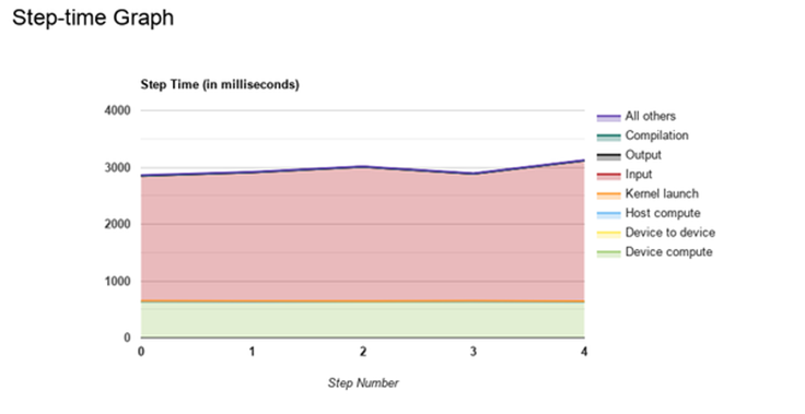
The model we will use is deep convolutional network that learns to perform pixel level segmentation on an input image. Our base model parallelizes the CPU and GPU processing and runs with a batch size of 64. In this case the training throughput is roughly 100 samples per second. The SageMaker dashboard reports GPU memory utilization of 98% and GPU utilization of between 95% and 100%.

我们将使用的模型是深度卷积网络，该网络将学习对输入图像执行像素级分割。 我们的基本模型并行化CPU和GPU处理，并以64的批处理大小运行。在这种情况下，训练吞吐量约为每秒100个样本。 SageMaker仪表板报告的GPU内存利用率为98％，GPU利用率为95％至100％。

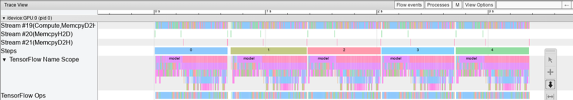
The efficiency of the GPU utilization can also be seen from the trace_viewer of the tf profiler where we can see that the GPU is almost always active. Recall that the tf profile was configured to run for five steps, steps 20–24.

您还可以从tf分析器的trace_viewer中看到GPU的利用效率，在这里我们可以看到GPU几乎始终处于活动状态。 回想一下，tf配置文件已配置为运行五个步骤，即步骤20-24。

tf profiler — trace-viewer (by author using TensorBoard)

tf profiler —跟踪查看器(作者使用TensorBoard)

For the sake of comparison, we will also note that the Instance Metrics reports network-in of 14.9 GBytes per minute, and network-out of under 100 MBytes per minute.

为了进行比较，我们还将注意到，“实例指标”报告的入网速度为每分钟14.9 GB，出网速度为每分钟100 MB以下。

小批量 (Small Batch Size)

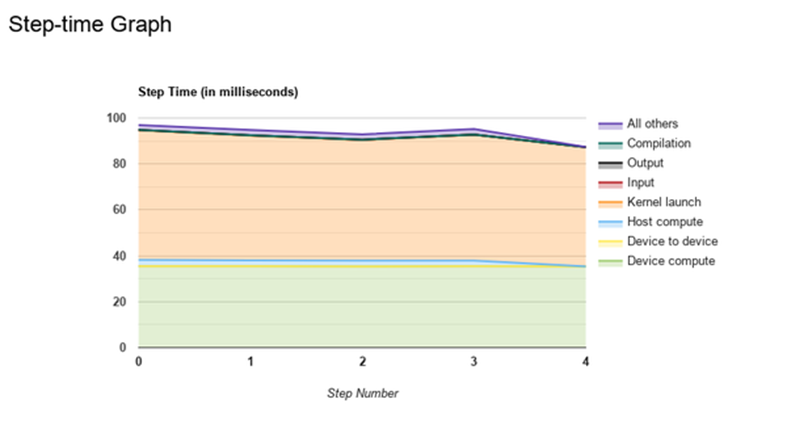
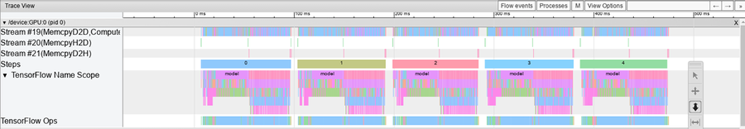
To evaluate the impact of the batch size on the performance, we reduce the batch size to 2, leaving all other model properties unchanged. The throughput drops all the way down to 40 samples per second. The effect on GPU utilization and GPU memory utilization is immediately noticeable from the “instance metrics” where we see a significant drop, down to around 60% and 23%, respectively. Naturally, each iteration takes a lot less time, but the percentage of the time during which the GPU is active is much lower.

为了评估批次大小对性能的影响，我们将批次大小减小为2，而所有其他模型属性均保持不变。 吞吐量一直下降到每秒40个样本。 从“实例指标”可以立即注意到对GPU利用率和GPU内存利用率的影响，我们发现该指标显着下降，分别降至约60％和23％。 自然地，每次迭代花费的时间要少得多，但是GPU处于活动状态的时间百分比要低得多。

The tf profiler step time graph shows that the small batch size leads to over half the time being spent loading kernels to the GPU.

tf探查器步骤时间图显示，小批处理量导致将内核加载到GPU所花费的时间超过一半。

Small Batch Size — tf profiler Step-time Graph (by author using TensorBoard)

小批量-tf探查器步进图(作者使用TensorBoard)

The trace_viewer shows that while the GPU remains unblocked by the input, the tf ops appear to be sparsely scattered across the computation block of each step.

trace_viewer显示，尽管GPU不受输入的限制，但tf ops似乎稀疏地分散在每个步骤的计算块中。

Small Batch Size — tf profiler trace-viewer (by author using TensorBoard)

小批量— tf分析器跟踪查看器(作者使用TensorBoard)

In TensorFlow 2.3, a new Memory profiler tool was introduced that allows you to identify under utilization of the GPU memory and get an indication of whether you can safely increase the training batch size.

在TensorFlow 2.3中，引入了新的Memory Profiler工具，该工具可让您识别GPU内存的利用率是否不足，并指示您是否可以安全地增加训练批次的大小。

网络输入瓶颈 (Network Input Bottleneck)

In this example, we will artificially introduce a network bottleneck on the network input. We will do this by dropping every 9 out 10 input records so that we require 10 times as much input data on the network to maintain the same throughput. Here is the code used to perform this exercise:

在此示例中，我们将在网络输入上人为地引入网络瓶颈。 我们将通过删除10条输入记录中的每9条记录来做到这一点，以便我们在网络上需要10倍的输入数据来维持相同的吞吐量。 这是用于执行此练习的代码：

# id generatordef id_gen():
    e = 0
    while True:
        yield e
        e += 1# enter id to feature dictdef add_id_label(f, i):
    f['id'] = i
    return f# create a dataset of indices and zip it with input datasetids = tf.data.Dataset.from_generator(id_gen, tf.int64)
ds = tf.data.Dataset.zip((ds, ids))# enter id to feature dictds = ds.map(add_id_label, num_parallel_calls=tf.data.experimental.autotune)# filter out every 9 out of 10 recordsds = ds.filter(lambda f: 
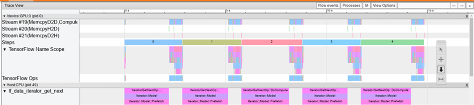
               tf.squeeze(tf.equal(tf.math.floormod(f['id'],10),0)))

From the instance metrics, we can see that the network-in caps out at 33.4 GBytes per minute, only a bit more than twice the volume of the normal run (14.9 GBytes) despite the fact that we need ten times as much data. Throughput drops to 22 samples per second. Unsurprisingly, our program is highly input bound. The tf profiler reports that, of the total step time, 77.8% is spent waiting for data.

从实例指标中，我们可以看到，入网速度为每分钟33.4 GB，尽管我们需要十倍的数据量，但仅比正常运行(14.9 GB)多两倍。 吞吐量下降到每秒22个样本。 毫不奇怪，我们的程序具有很高的输入范围。 tf分析器报告说，在总的步骤时间中，等待数据花费了77.8％。

NetworkIn Bottleneck — tf profiler Step-time Graph (by author using TensorBoard)

NetworkIn瓶颈— tf探查器步进时间图(作者使用TensorBoard)

The trace_viewer clearly shows the GPU sitting idle for the majority of each step as it waits for data from the tf_data_iterator_get_next op.

trace_viewer清楚地显示了GPU在等待来自tf_data_iterator_get_next op的数据时大部分时间处于空闲状态。

NetworkIn Bottleneck — tf profiler trace-viewer (by author using TensorBoard)

NetworkIn瓶颈— tf探查器跟踪查看器(作者使用TensorBoard)

预处理管道超载 (Overloaded Pre-processing Pipeline)

TensorFlow offers ways to maximize the parallelization of the data processing (as demonstrated in the TensorBoard Profiler Tutorials) but this does not absolve you from optimizing your input data processing pipeline. If your data processing is resource intensive, it may impact the performance of your model, and you might want to consider moving some of your processing offline. If the heavy operation is GPU friendly, (e.g. a large convolution), you can also consider performing the operation on the GPU using the experimental map_on_gpu function, (but keep in mind the overhead of the data transfer). Another option is to choose a training instance with more CPU cores.

TensorFlow提供了最大化数据处理并行化的方法(如TensorBoard Profiler教程所示 )，但这并不能免除您优化输入数据处理管道的麻烦 。 如果您的数据处理占用大量资源，则可能会影响模型的性能，并且您可能需要考虑将某些处理脱机。 如果繁重的操作是GPU友好的(例如，大卷积)，则您也可以考虑使用实验性map_on_gpu函数在GPU上执行操作(但要记住数据传输的开销)。 另一个选择是选择具有更多CPU内核的训练实例。

In this example, we will simulate an overloaded pre-processing pipeline, by applying a separable_conv2d with filter size 7x7 to the input frame.

在此示例中，我们将通过将过滤器大小为7x7的separable_conv2d应用于输入帧，来模拟过载的预处理管道。

The throughput drops to just 25 samples per second, and the maximum GPU utilization to 36%. The CPU utilization, on the other hand, jumps from 66% to 96%. Once again, the program is highly input bound, and the trace-viewer shows large chunks of GPU idle time.

吞吐量下降到每秒仅25个样本，最大GPU利用率下降到36％。 另一方面，CPU利用率从66％跃升至96％。 程序再次受到高输入限制，跟踪查看器显示了大量的GPU空闲时间。

Preproc Bottleneck — tf profiler trace-viewer (by author using TensorBoard)

Preproc瓶颈— tf分析器跟踪查看器(作者使用TensorBoard)

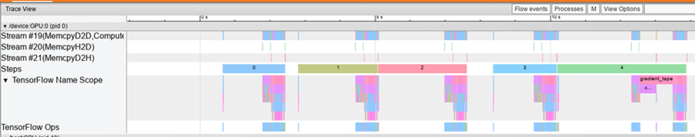
Careful analysis of the CPU section of the trace-viewer, (not shown here), shows that separable convolution taking up large chunks of the compute.

仔细分析跟踪查看器的CPU部分(此处未显示)，可分离的卷积占用了很大的计算量。

CPU GPU数据接口的瓶颈 (Bottleneck on CPU GPU data Interface)

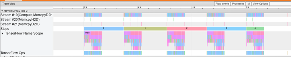
In this example, we artificially increase the input data being passed to the GPU by blowing up the size of the input frame by a factor of 10. On the CPU side we simply replicate the input frame 10 times (using tf.tile()). On the GPU we receive the enlarged input frame, but immediately discard the added data.

在此示例中，我们通过将输入帧的大小放大了10倍来人为地增加了传递到GPU的输入数据。在CPU端，我们只需将输入帧复制10次(使用tf.tile()) 。 在GPU上，我们接收到放大的输入帧，但立即丢弃添加的数据。

The throughput in this case drops to 84 samples per second, and the bottleneck is clearly evident on the trace-viewer.

在这种情况下，吞吐量下降到每秒84个样本，并且在跟踪查看器上明显可见瓶颈。

H2D bottleneck — tf profiler trace-viewer (by author using TensorBoard)

H2D瓶颈— TF Profiler跟踪查看器(作者使用TensorBoard编写)

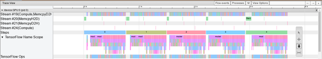
Notice how, for each step, the size of the block of Stream #20(MemcpyH2D) has grown, and how the GPU compute remains idle until the block has completed.

请注意，对于每个步骤， 流＃20(MemcpyH2D)的块大小如何增大 ，以及GPU计算如何保持空闲，直到该块完成为止。

GPU效率低下 (Inefficiency in GPU)

In this example, we simulate the impact of an inefficient graph, by applying an 11x11 convolution filter to the output of the model before calculating the loss function. Unsurprisingly, the throughput drops slightly, to 96 samples per second. The impact on the graph can be viewed on the tf profiler tensorflow stats page, where we see that the added operation becomes the most time-consuming operation in the GPU. This table gives us information on the heaviest operations, which we can use to improve the model performance.

In this example, we simulate the impact of an inefficient graph, by applying an 11x11 convolution filter to the output of the model before calculating the loss function. Unsurprisingly, the throughput drops slightly, to 96 samples per second. The impact on the graph can be viewed on the tf profiler tensorflow stats page, where we see that the added operation becomes the most time-consuming operation in the GPU. This table gives us information on the heaviest operations, which we can use to improve the model performance.

Inefficient Graph — tensorflow stats (by author using TensorBoard)

Inefficient Graph — tensorflow stats (by author using TensorBoard)

Heavy Post Processing (Heavy Post Processing)

In this example, we add a callback function that simulates processing the segmentation masks that are output by the model, by creating and storing 64 random images after every iteration. The first thing we notice, is that TensorFlow prints the following warning:

In this example, we add a callback function that simulates processing the segmentation masks that are output by the model, by creating and storing 64 random images after every iteration. The first thing we notice, is that TensorFlow prints the following warning:

WARNING:tensorflow:Method (on_train_batch_end) is slow compared to the batch update (0.814319). Check your callbacks.

Additionally, the throughput drops to 43 samples per second, the GPU utilization drops to 46%, and tf profiler reports that the GPU is active for only 47% of each time step. The bottleneck is clearly seen on the trace-viewer where we see the GPU idle for the second half of each step.

Additionally, the throughput drops to 43 samples per second, the GPU utilization drops to 46%, and tf profiler reports that the GPU is active for only 47% of each time step. The bottleneck is clearly seen on the trace-viewer where we see the GPU idle for the second half of each step.

Postproc Bottleneck — tf profiler trace-viewer (by author using TensorBoard)

Postproc Bottleneck — tf profiler trace-viewer (by author using TensorBoard)

摘要 (Summary)

As we have shown, the ability to analyze and optimize the performance of your training sessions, can lead to meaningful savings in time and cost. The skills required to perform such analysis should exist in your DNN development team. The analysis should be an integral part of your team’s development methodology and incorporated into your DNN training life cycle. Your development plan should include details such, as at when to run performance profiling, what tools to use, what type of tests to run, how invasive the tests should be, and more.

As we have shown, the ability to analyze and optimize the performance of your training sessions, can lead to meaningful savings in time and cost. The skills required to perform such analysis should exist in your DNN development team. The analysis should be an integral part of your team's development methodology and incorporated into your DNN training life cycle. Your development plan should include details such, as at when to run performance profiling, what tools to use, what type of tests to run, how invasive the tests should be, and more.

In this post we have barely touched the surface of the world of performance analysis. There are, no doubt, many more tools and techniques, other kinds of bottlenecks, and other ways to squeeze more performance out of your training resources. Our goal was merely to introduce you into this world, and emphasize its importance in your day to day training. Best of luck to you!!

In this post we have barely touched the surface of the world of performance analysis. There are, no doubt, many more tools and techniques, other kinds of bottlenecks, and other ways to squeeze more performance out of your training resources. Our goal was merely to introduce you into this world, and emphasize its importance in your day to day training. Best of luck to you!!

翻译自: https://towardsdatascience.com/tensorflow-performance-analysis-314b56dceb59