逻辑回归画图_逻辑回归

逻辑回归画图

申请流程 (Application Flow)

Logistic Regression is one of the most fundamental algorithms for classification in the Machine Learning world.

Logistic回归是机器学习世界中分类的最基本算法之一。

But before proceeding with the algorithm, let’s first discuss the lifecycle of any machine learning model. This diagram explains the creation of a Machine Learning model from scratch and then taking the same model further with hyperparameter tuning to increase its accuracy, deciding the deployment strategies for that model and once deployed setting up the logging and monitoring frameworks to generate reports and dashboards based on the client requirements. A typical lifecycle diagram for a machine learning model looks like:

但是在继续算法之前，让我们首先讨论任何机器学习模型的生命周期。 该图说明了从头开始创建机器学习模型的过程，然后通过超参数调整进一步推广了该模型，以提高其准确性，确定了该模型的部署策略，并在部署后设置了日志记录和监视框架以生成基于报告和仪表板的信息。根据客户要求。 机器学习模型的典型生命周期图如下所示：

介绍 (Introduction)

In linear regression, the type of data we deal with is quantitative, whereas we use classification models to deal with qualitative data or categorical data. The algorithms used for solving a classification problem first predict the probability of each of the categories of the qualitative variables, as the basis for making the classification. And, as the probabilities are continuous numbers, classification using probabilities also behave like regression methods. Logistic regression is one such type of classification model which is used to classify the dependent variable into two or more classes or categories.

在线性回归中，我们处理的数据类型是定量的，而我们使用分类模型来处理定性数据或分类数据。 用于解决分类问题的算法首先预测定性变量的每个类别的概率，作为进行分类的基础。 并且，由于概率是连续数，因此使用概率进行分类的行为也类似于回归方法。 逻辑回归是一种这样的分类模型，用于将因变量分为两个或多个类别或类别。

Why don’t we use Linear regression for classification problems?

为什么我们不对分类问题使用线性回归？

Let’s suppose you took a survey and noted the response of each person as satisfied, neutral or Not satisfied. Let’s map each category:

假设您进行了一项调查，并注意到每个人的回答为满意，中立或不满意。 让我们映射每个类别：

Satisfied — 2

满意— 2

Neutral — 1

中立— 1

Not Satisfied — 0

不满意— 0

But this doesn’t mean that the gap between Not satisfied and Neutral is same as Neutral and satisfied. There is no mathematical significance of these mapping. We can also map the categories like:

但这并不意味着不满意和中立之间的差距与中立和满意之间的差距相同。 这些映射没有数学意义。 我们还可以映射以下类别：

Satisfied — 0

满意— 0

Neutral — 1

中立— 1

Not Satisfied — 2

不满意— 2

It’s completely fine to choose the above mapping. If we apply linear regression to both the type of mappings, we will get different sets of predictions. Also, we can get prediction values like 1.2, 0.8, 2.3 etc. which makes no sense for categorical values. So, there is no normal method to convert qualitative data into quantitative data for use in linear regression. Although, for binary classification, i.e. when there only two categorical values, using the least square method can give decent results. Suppose we have two categories Black and White and we map them as follows:

选择上面的映射是完全可以的。 如果将线性回归应用于这两种映射类型，我们将获得不同的预测集。 同样，我们可以获得诸如1.2、0.8、2.3等的预测值，这对于分类值没有意义。 因此，没有正常的方法可以将定性数据转换为定量数据以用于线性回归。 虽然，对于二进制分类，即当只有两个分类值时，使用最小二乘法可以得到不错的结果。 假设我们有黑色和白色两个类别，我们将它们映射如下：

Black — 0

黑色— 0

White — 1

白色— 1

We can assign predicted values for both the categories such as Y> 0.5 goes to class white and vice versa. Although, there will be some predictions for which the value can be greater than 1 or less than 0 making them hard to classify in any class. Nevertheless, linear regression can work decently for binary classification but not that well for multi-class classification. Hence, we use classification methods for dealing with such problems.

我们可以为这两个类别分配预测值，例如Y> 0.5归为白色类别，反之亦然。 虽然，有些预测的值可能大于1或小于0，这使得它们很难在任何类别中进行分类。 然而，线性回归对于二元分类可以很好地工作，但对于多分类则不能很好地工作。 因此，我们使用分类方法来处理此类问题。

逻辑回归 (Logistic Regression)

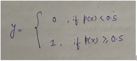
Logistic regression is one such regression algorithm which can be used for performing classification problems. It calculates the probability that a given value belongs to a specific class. If the probability is more than 50%, it assigns the value in that particular class else if the probability is less than 50%, the value is assigned to the other class. Therefore, we can say that logistic regression acts as a binary classifier.

逻辑回归是一种可以用于执行分类问题的回归算法。 它计算给定值属于特定类别的概率。 如果概率大于50％，则在该特定类别中分配值，否则，如果概率小于50％，则将该值分配给另一类别。 因此，可以说逻辑回归充当二进制分类器。

Working of a Logistic Model

物流模型的工作

For linear regression, the model is defined by: 𝑦=𝛽0+𝛽1𝑥y=β0+β1x — (i)

对于线性回归，模型定义为：𝑦= 𝛽0 + 𝛽1𝑥y =β0+β1x—(i)

and for logistic regression, we calculate probability, i.e. y is the probability of a given variable x belonging to a certain class. Thus, it is obvious that the value of y should lie between 0 and 1.

对于逻辑回归，我们计算概率，即y是给定变量x属于某个类别的概率。 因此，很明显，y的值应该在0到1之间。

But, when we use equation(i) to calculate probability, we would get values less than 0 as well as greater than 1. That doesn’t make any sense . So, we need to use such an equation which always gives values between 0 and 1, as we desire while calculating the probability.

但是，当我们使用方程式(i)计算概率时，我们将获得小于0且大于1的值。这没有任何意义。 因此，我们需要使用这样的方程式，该方程式总是根据需要在计算概率时给出介于0和1之间的值。

乙状结肠功能 (Sigmoid function)

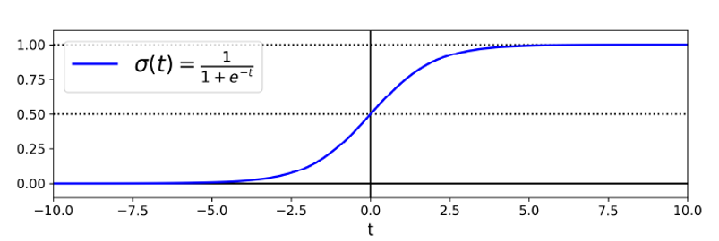
We use the sigmoid function as the underlying function in Logistic regression. Mathematically and graphically, it is shown as:

我们将S形函数用作Logistic回归的基础函数。 在数学和图形上显示为：

Why do we use the Sigmoid Function?

为什么要使用Sigmoid函数？

1) The sigmoid function’s range is bounded between 0 and 1. Thus it’s useful in calculating the probability for the Logistic function. 2) It’s derivative is easy to calculate than other functions which is useful during gradient descent calculation. 3) It is a simple way of introducing non-linearity to the model.

1)S形函数的范围在0到1之间。因此，在计算Logistic函数的概率时很有用。 2)它的导数比其他函数容易计算，这在梯度下降计算中很有用。 3)这是将非线性引入模型的简单方法。

Although there are other functions as well, which can be used, but sigmoid is the most common function used for logistic regression. We will talk about the rest of the functions in the neural network section.

尽管还可以使用其他函数，但是Sigmoid是用于Logistic回归的最常用函数。 我们将在神经网络部分讨论其余功能。

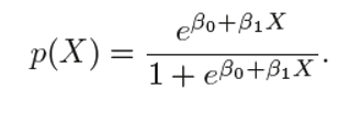
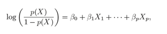
The logistic function is given as:

逻辑函数为：

Let’s see some manipulation with the logistic function:

让我们看一下使用logistic函数的一些操作：

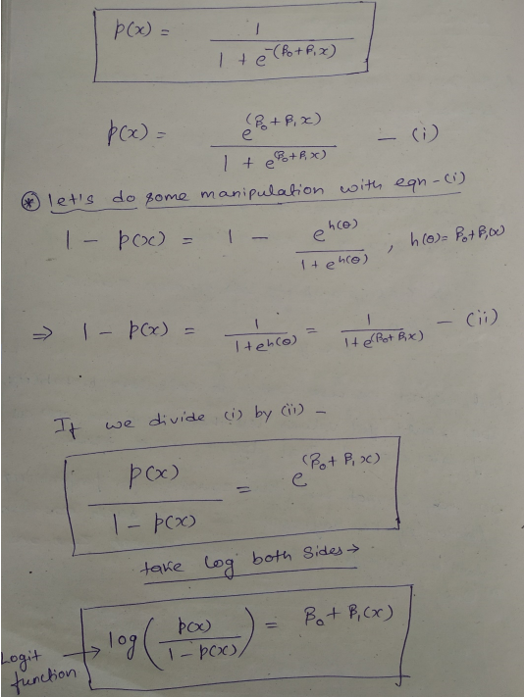
We can see that the logit function is linear in terms with x.

我们可以看到logit函数与x呈线性关系。

Prediction

预测

Cost Function

成本函数

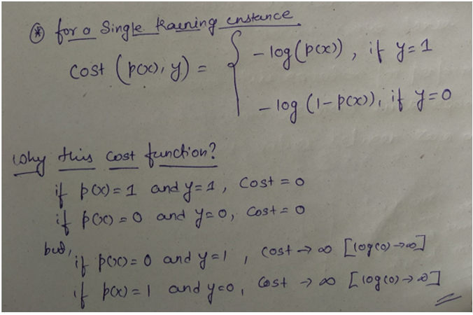
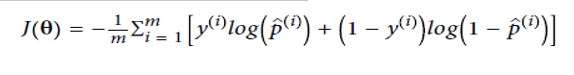
The cost function for the whole training set is given as :

整个训练集的成本函数为：

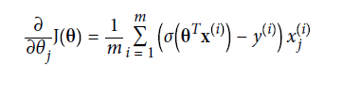
The values of parameters (θ) for which the cost function is minimum is calculated using the gradient descent (as discussed in the Linear Regression section) algorithm. The partial derivative for cost function is given as :

使用梯度下降(如“线性回归”部分所述)算法来计算成本函数最小的参数(θ)的值。 成本函数的偏导数为：

多种物流功能 (Multiple Logistic Function)

We can generalise the simple logistic function for multiple features as:

我们可以将简单的逻辑函数推广为多种功能，如：

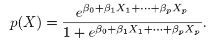
And the logit function can be written as:

logit函数可以写成：

he coefficients are calculated the same we did for simple logistic function, by passing the above equation in the cost function.

通过将上述方程式传递给成本函数，系数的计算方法与简单逻辑函数相同。

Just like we did in multilinear regression, we will check for correlation between different features for Multi logistic as well.

就像我们在多线性回归中所做的一样，我们还将为Multi logistic检查不同特征之间的相关性。

We will see how we implement all the above concept through a practical example.

我们将通过一个实际示例来了解如何实现上述所有概念。

多项式物流回归(标签数量> 2) (Multinomial Logistics Regression( Number of Labels >2))

Many times, there are classification problems where the number of classes is greater than 2. We can extend Logistic regression for multi-class classification. The logic is simple; we train our logistic model for each class and calculate the probability(hθx) that a specific feature belongs to that class. Once we have trained the model for all the classes, we predict a new value’s class by choosing that class for which the probability(hθx) is maximum. Although we have libraries that we can use to perform multinomial logistic regression, we rarely use logistic regression for classification problems where the number of classes is more than 2. There are many other classification models for such scenarios. We will see more of that in the coming lectures.

很多时候，存在类别数大于2的分类问题。我们可以扩展Logistic回归进行多类别分类。 逻辑很简单； 我们为每个类别训练逻辑模型，并计算特定特征属于该类别的概率(hθx)。 一旦我们为所有类别训练了模型，就可以通过选择概率(hθx)最大的类别来预测新值的类别。 尽管我们拥有可用于执行多项式logistic回归的库，但是对于类数大于2的分类问题，我们很少使用logistic回归。对于这种情况，还有许多其他分类模型。 我们将在接下来的讲座中看到更多。

学习算法 (Learning Algorithm)

The learning algorithm is how we search the set of possible hypotheses (hypothesis space H) for the best parameterization (in this case the weight vector 𝐰w). This search is an optimization problem looking for the hypothesis that optimizes an error measure.

学习算法是我们如何搜索可能的假设集(假设空间H)以获得最佳参数化(在这种情况下为权重向量𝐰w)。 该搜索是一个优化问题，用于寻找优化错误度量的假设。

There is no sophisticted, closed-form solution like least-squares linear, so we will use gradient descent instead. Specifically we will use batch gradient descent which calculates the gradient from all data points in the data set.

没有像最小二乘线性这样的复杂的封闭形式的解决方案，因此我们将使用梯度下降。 具体来说，我们将使用批量梯度下降，它从数据集中的所有数据点计算梯度。

Luckily, our “cross-entropy” error measure is convex so there is only one minimum. Thus the minimum we arrive at is the global minimum.

幸运的是，我们的“交叉熵”误差度量是凸的，因此只有一个最小值。 因此，我们得出的最小值是全局最小值。

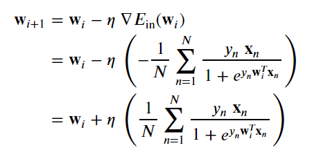
To learn we’re going to minimize the following error measure using batch gradient descent.

要学习，我们将使用批量梯度下降来最小化以下误差度量。

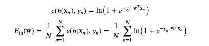
We’ll need the derivative of the point loss function and possibly some abuse of notation.

我们将需要点损失函数的导数，并且可能需要滥用符号。

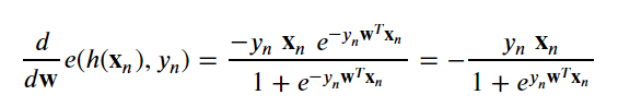
With the point loss derivative we can determine the gradient of the in-sample error:

利用点损失导数，我们可以确定样本内误差的梯度：

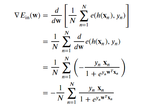
Our weight update rule per batch gradient descent becomes

我们每批次梯度下降的重量更新规则变为

分类模型评估 (Evaluation of a Classification Model)

In machine learning, once we have a result of the classification problem, how do we measure how accurate our classification is? For a regression problem, we have different metrics like R Squared score, Mean Squared Error etc. what are the metrics to measure the credibility of a classification model?

在机器学习中，一旦有了分类问题的结果，我们如何衡量分类的准确性？ 对于回归问题，我们有不同的指标，例如R平方得分，均方误差等。衡量分类模型可信度的指标是什么？

Metrics In a regression problem, the accuracy is generally measured in terms of the difference in the actual values and the predicted values. In a classification problem, the credibility of the model is measured using the confusion matrix generated, i.e., how accurately the true positives and true negatives were predicted. The different metrics used for this purpose are:

度量标准在回归问题中，通常根据实际值和预测值之间的差异来测量准确性。 在分类问题中，使用生成的混淆矩阵来衡量模型的可信度，即，如何准确预测正值和负值。 用于此目的的不同指标是：

• Accuracy
  准确性
• Recall
  召回
• Precision
  精确
• F1 Score
  F1分数
• Specifity
  特异性
• AUC( Area Under the Curve)
  AUC(曲线下面积)
• RUC(Receiver Operator Characteristic)
  RUC(接收机操作员特性)

混淆矩阵 (Confusion Matrix)

A typical confusion matrix looks like the figure shown.

典型的混淆矩阵看起来如图所示。

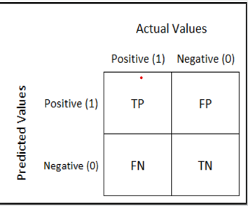
Where the terms have the meaning:

术语含义如下：

 True Positive(TP): A result that was predicted as positive by the classification model and also is positive

 真实阳性(TP)：分类模型预测为阳性的结果，也是阳性的

 True Negative(TN): A result that was predicted as negative by the classification model and also is negative

 真负数(TN)：分类模型预测为负数且也是负数的结果

 False Positive(FP): A result that was predicted as positive by the classification model but actually is negative

Positive假阳性(FP)：分类模型预测为阳性但实际上为阴性的结果

 False Negative(FN): A result that was predicted as negative by the classification model but actually is positive.

 假阴性(FN)：分类模型预测为阴性但实际上为阳性的结果。

The Credibility of the model is based on how many correct predictions did the model do.

模型的可信度基于模型进行了多少正确的预测。

准确性 (Accuracy)

The mathematical formula is :

数学公式为：

Accuracy= (𝑇𝑃+𝑇𝑁)(𝑇𝑃+𝑇𝑁+𝐹𝑃+𝐹𝑁)(TP+TN)(TP+TN+FP+FN)

精度 =(𝑇𝑃+𝑇𝑁)(𝑇𝑃+𝑇𝑁+𝐹𝑃+𝐹𝑁)(TP + TN)(TP + TN + FP + FN)

Or, it can be said that it’s defined as the total number of correct classifications divided by the total number of classifications.

或者，可以说它定义为正确分类的总数除以分类的总数。

召回或敏感性 (Recall or Sensitivity)

The mathematical formula is:

数学公式为：

Recall= 𝑇𝑃(𝑇𝑃+𝐹𝑁)TP(TP+FN)

召回率 =𝑇𝑃(𝑇𝑃+𝐹𝑁)TP(TP + FN)

Or, as the name suggests, it is a measure of: from the total number of positive results how many positives were correctly predicted by the model.

或者，顾名思义，它是一种度量：从阳性结果总数中，模型可以正确预测多少阳性。

It shows how relevant the model is, in terms of positive results only.

它仅根据正面结果显示了该模型的相关性。

Let’s suppose in the previous model, the model gave 50 correct predictions(TP) but failed to identify 200 cancer patients(FN). Recall in that case will be:

让我们假设在先前的模型中，该模型给出了50个正确的预测(TP)，但未能识别200位癌症患者(FN)。 在这种情况下，回想一下：

Recall=50(50+200)50(50+200)= 0.2 (The model was able to recall only 20% of the cancer patients)

召回率= 50(50 + 200)50(50 + 200)= 0.2(该模型仅能召回20％的癌症患者)

精确 (Precision)

Precision is a measure of amongst all the positive predictions, how many of them were actually positive. Mathematically,

精确度是对所有积极预测中，实际上有多少是积极衡量的一种度量。 数学上

Precision=𝑇𝑃(𝑇𝑃+𝐹𝑃)TP(TP+FP)

精度=𝑇𝑃(𝑇𝑃+𝐹𝑃)TP(TP + FP)

Let’s suppose in the previous example, the model identified 50 people as cancer patients(TP) but also raised a false alarm for 100 patients(FP). Hence,

让我们假设在前面的示例中，该模型将50个人确定为癌症患者(TP)，但还对100位患者提出了虚警(FP)。 因此，

Precision=50(50+100)50(50+100)=0.33 (The model only has a precision of 33%)

精度= 50(50 + 100)50(50 + 100)= 0.33(该模型的精度仅为33％)

但是我们有一个问题！ (But we have a problem!!)

As evident from the previous example, the model had a very high Accuracy but performed poorly in terms of Precision and Recall. So, necessarily Accuracy is not the metric to use for evaluating the model in this case.

从前面的示例可以明显看出，该模型具有很高的准确度，但在“精确度”和“查全率”方面却表现不佳。 因此，在这种情况下， 精度不一定是用于评估模型的度量。

Imagine a scenario, where the requirement was that the model recalled all the defaulters who did not pay back the loan. Suppose there were 10 such defaulters and to recall those 10 defaulters, and the model gave you 20 results out of which only the 10 are the actual defaulters. Now, the recall of the model is 100%, but the precision goes down to 50%.

想象一下一个场景，该场景的要求是模型召回所有未偿还贷款的违约者。 假设有10个这样的默认违约者，并回忆起这10个默认违约者，该模型为您提供了20个结果，其中只有10个是实际的默认违约者。 现在，该模型的召回率为100％，但精度下降到50％。

权衡？ (A Trade-off?)

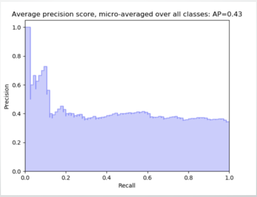
As observed from the graph, with an increase in the Recall, there is a drop in Precision of the model.

从图表中可以看出，随着查全率的增加，模型的精确度会下降。

So the question is — what to go for? Precision or Recall?

因此，问题是-去做什么？ 精度还是召回率？

Well, the answer is: it depends on the business requirement.

好吧，答案是：这取决于业务需求。

For example, if you are predicting cancer, you need a 100 % recall. But suppose you are predicting whether a person is innocent or not, you need 100% precision.

例如，如果您要预测癌症，则需要100％召回。 但是，假设您要预测一个人是否清白，则需要100％的精度。

Can we maximise both at the same time? No

我们可以同时最大化两者吗？ 没有

So, there is a need for a better metric then?

那么，是否需要更好的指标？

Yes. And it’s called an F1 Score

是。 这就是所谓的F1分数

F1分数 (F1 Score)

From the previous examples, it is clear that we need a metric that considers both Precision and Recall for evaluating a model. One such metric is the F1 score.

从前面的示例中可以明显看出，我们需要一个同时考虑Precision和Recall的度量来评估模型。 F1分数就是此类指标之一。

F1 score is defined as the harmonic mean of Precision and Recall.

F1分数定义为“精确度”和“查全率”的谐波平均值。

The mathematical formula is: F1 score= 2∗((𝑃𝑟𝑒𝑐𝑖𝑠𝑖𝑜𝑛∗𝑅𝑒𝑐𝑎𝑙𝑙)(𝑃𝑟𝑒𝑐𝑖𝑠𝑖𝑜𝑛+𝑅𝑒𝑐𝑎𝑙𝑙))2∗((Precision∗Recall)(Precision+Recall))

数学公式为：F1分数= 2 ∗(((𝑃𝑟𝑒𝑐𝑖𝑠𝑖𝑜𝑛∗𝑅𝑒𝑐𝑎𝑙𝑙)(𝑃𝑟𝑒𝑐𝑖𝑠𝑖𝑜𝑛+𝑅𝑒𝑐𝑎𝑙𝑙))2 ∗((Precision ∗ Recall)(Precision + Recall))

特异性或真阴性率 (Specificity or True Negative Rate)

This represents how specific is the model while predicting the True Negatives. Mathematically,

这代表了在预测真实负面因素时模型的特异性。 数学上

Specificity=𝑇𝑁(𝑇𝑁+𝐹𝑃)TN(TN+FP) Or, it can be said that it quantifies the total number of negatives predicted by the model with respect to the total number of actual negative or non favorable outcomes.

特异性=𝑇𝑁(𝑇𝑁+𝐹𝑃)TN(TN + FP)或者，可以说，相对于实际阴性或不利结果的总数，量化了模型预测的阴性总数。

Similarly, False Positive rate can be defined as: (1- specificity) Or, 𝐹𝑃(𝑇𝑁+𝐹𝑃)FP(TN+FP)

类似地，误报率可以定义为：(1-特异性)或𝐹𝑃(𝑇𝑁+𝐹𝑃)FP(TN + FP)

ROC(接收机操作员特性) (ROC(Receiver Operator Characteristic))

We know that the classification algorithms work on the concept of probability of occurrence of the possible outcomes. A probability value lies between 0 and 1. Zero means that there is no probability of occurrence and one means that the occurrence is certain.

我们知道分类算法是基于可能结果出现概率的概念。 概率值在0到1之间。零表示没有发生的可能性，而一表示发生的可能性是确定的。

But while working with real-time data, it has been observed that we seldom get a perfect 0 or 1 value. Instead of that, we get different decimal values lying between 0 and 1. Now the question is if we are not getting binary probability values how are we actually determining the class in our classification problem?

但是，在处理实时数据时，已经观察到我们很少获得完美的0或1值。 取而代之的是，我们获得了介于0和1之间的不同十进制值。现在的问题是，如果我们没有获得二进制概率值，那么我们如何确定分类问题中的类别呢？

There comes the concept of Threshold. A threshold is set, any probability value below the threshold is a negative outcome, and anything more than the threshold is a favourable or the positive outcome. For Example, if the threshold is 0.5, any probability value below 0.5 means a negative or an unfavourable outcome and any value above 0.5 indicates a positive or favourable outcome.

阈值的概念。 设置了阈值，低于该阈值的任何概率值都是负结果，超过该阈值的任何值都是有利或积极结果。 例如，如果阈值为0.5，则任何低于0.5的概率值都表示结果为负或不利，而高于0.5的任何值都表示结果为正或有利。

Now, the question is, what should be an ideal threshold?

现在的问题是，理想的阈值应该是多少？

The following diagram shows a typical logistic regression curve.

下图显示了典型的逻辑回归曲线。

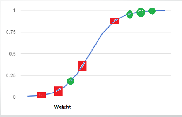
• The horizontal lines represent the various values of thresholds ranging from 0 to 1.
  水平线代表阈值的各种值，范围从0到1。
• Let’s suppose our classification problem was to identify the obese people from the given data.
  假设我们的分类问题是从给定的数据中识别肥胖者。
• The green markers represent obese people and the red markers represent the non-obese people.
  绿色标记代表肥胖的人，红色标记代表非肥胖的人。
• Our confusion matrix will depend on the value of the threshold chosen by us.
  我们的混淆矩阵将取决于我们选择的阈值。
• For Example, if 0.25 is the threshold then
  例如，如果阈值为0.25，则

TP(actually obese)=3 TN(Not obese)=2 FP(Not obese but predicted obese)=2(the two red squares above the 0.25 line) FN(Obese but predicted as not obese )=1(Green circle below 0.25line ) (TP(actually obese)=3 TN(Not obese)=2 FP(Not obese but predicted obese)=2(the two red squares above the 0.25 line) FN(Obese but predicted as not obese )=1(Green circle below 0.25line ))

A typical ROC curve looks like the following figure.

典型的ROC曲线如下图所示。

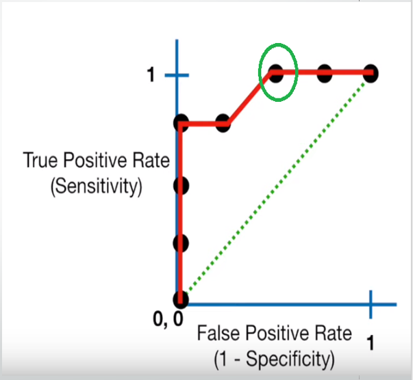
• Mathematically, it represents the various confusion matrices for various thresholds. Each black dot is one confusion matrix.
  从数学上讲，它代表各种阈值的各种混淆矩阵。 每个黑点都是一个混淆矩阵。
• The green dotted line represents the scenario when the true positive rate equals the false positive rate.
  绿色虚线表示当真阳性率等于假阳性率时的情况。
• As evident from the curve, as we move from the rightmost dot towards left, after a certain threshold, the false positive rate decreases.
  从曲线可以明显看出，当我们从最右边的点向左边移动时，经过一定的阈值后，假阳性率会降低。
• After some time, the false positive rate becomes zero.
  一段时间后，误报率变为零。
• The point encircled in green is the best point as it predicts all the values correctly and keeps the False positive as a minimum.
  用绿色圈出的点是最佳点，因为它可以正确预测所有值，并使False正值保持最小。
• But that is not a rule of thumb. Based on the requirement, we need to select the point of a threshold.
  但这不是经验法则。 根据需求，我们需要选择阈值点。
• The ROC curve answers our question of which threshold to choose.
  ROC曲线回答了我们选择哪个阈值的问题。

但是我们很困惑！ (But we have confusion !!)

Let’s suppose that we used different classification algorithms, and different ROCs for the corresponding algorithms have been plotted. The question is: which algorithm to choose now? The answer is to calculate the area under each ROC curve.

假设我们使用了不同的分类算法，并且为相应的算法绘制了不同的ROC。 问题是：现在选择哪种算法？ 答案是计算每个ROC曲线下的面积。

曲线下面积 (AUC(Area Under Curve))

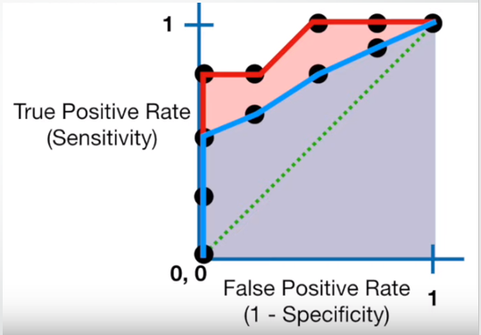
• It helps us to choose the best model amongst the models for which we have plotted the ROC curves
  它有助于我们在绘制了ROC曲线的模型中选择最佳模型
• The best model is the one which encompasses the maximum area under it.
  最好的模型是包含其下最大面积的模型。
• In the adjacent diagram, amongst the two curves, the model that resulted in the red one should be chosen as it clearly covers more area than the blue one
  在相邻的图中，在两条曲线之间，应选择导致红色曲线的模型，因为它显然比蓝色曲线覆盖的区域更大

翻译自: https://medium.com/@er.amansingh2019/logistic-regression-401b3a7723de

逻辑回归画图