pca 主成分分析_六分钟的主成分分析（PCA）的直观说明。

pca 主成分分析

Principle Component Analysis (PCA) is arguably a very difficult-to-understand topic for beginners in machine learning. Here, I will try my best to intuitively explain what it is, how the algorithm does what it does. This post assumes you have very basic knowledge of Linear Algebra like matrix multiplication, and vectors.

对于机器学习的初学者而言，主成分分析(PCA)可以说是一个很难理解的主题。 在这里，我将尽力直观地解释它的含义，算法的作用。 这篇文章假设您具有线性代数的基本知识，例如矩阵乘法和向量。

什么是PCA？ (What is PCA?)

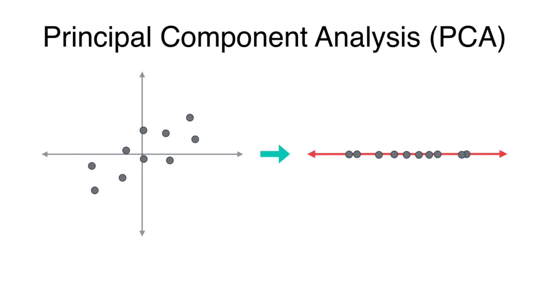
PCA is a dimensionality-reduction technique used to make large datasets with hundreds of thousands of features into smaller datasets with fewer features while retaining as much information about the dataset as possible.

P CA是一种降维技术，用于将具有数十万个特征的大型数据集制作为具有较少特征的较小数据集，同时保留有关该数据集的尽可能多的信息。

A perfect example would be:

一个完美的例子是：

Notice that in the original dataset there were five features which could be reduced to two features. These two features generalize the features on the left.

请注意，在原始数据集中有五个要素，可以简化为两个要素。 这两个功能概括了左侧的功能。

可视化PCA的想法。 (Visualizing the idea of PCA.)

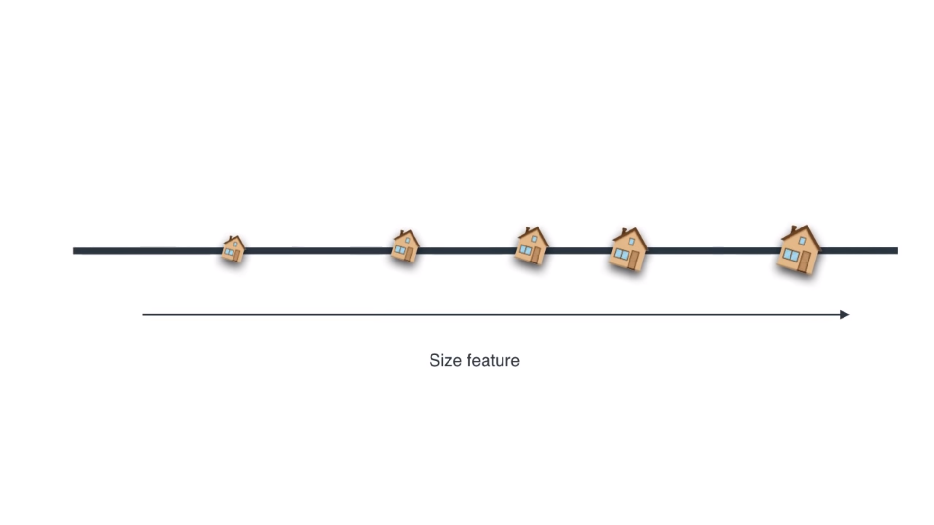
To make a picture of what’s happening, we use our previous example. A 2-dimensional plane showing the correlation of size to number of rooms in a house can be compressed to a single size feature, as shown below:

为了了解正在发生的事情，我们使用前面的示例。 可以将显示房屋大小与房间数量之间关系的二维平面压缩为单个尺寸特征，如下所示：

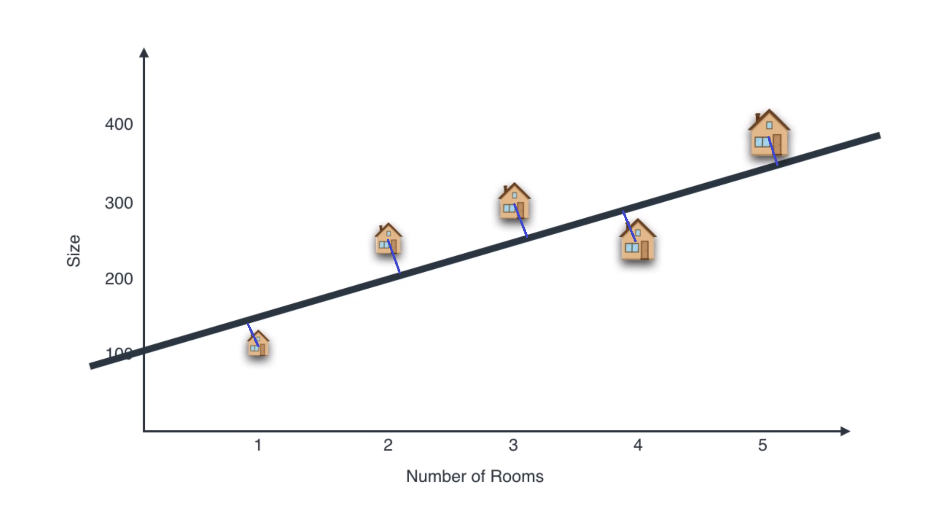
If we project the houses on the black line, we would get something like this:

如果我们将房屋投影在黑线上，我们将得到以下内容：

So we need to reduce that projection error (the magnitude of blue lines) in order to retain maximum information.

因此，我们需要减少投影误差(蓝线的大小)以保留最大的信息。

了解PCA算法的先决条件。 (Prerequisites to understanding the PCA Algorithm.)

I will explain some concepts intuitively in order for you to understand the algorithm better.

我将直观地解释一些概念，以使您更好地理解算法。

意思 (Mean)

Mean of any dataset refers to the equilibrium of the dataset. Imagine a rod on which balls are placed at some distance x from the wall:

任何数据集的均值是指数据集的平衡。 想象一下，一根杆上的球与墙之间的距离为x ：

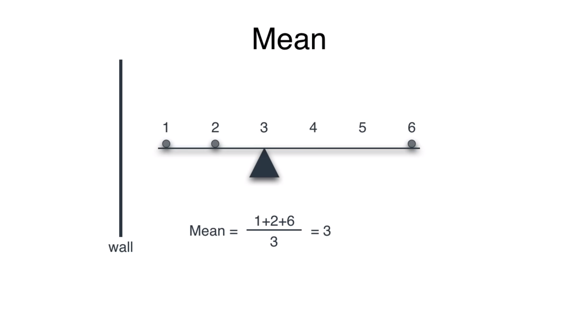
Summing the distance of the balls from the wall and dividing by the number of balls results the point of equilibrium, where a pivot would balance the rod.

将球与壁的距离相加并除以球的数量可得出平衡点，在该点上，枢轴将平衡杆。

方差 (Variance)

Mean tells us about the equilibrium of the dataset, variance is a metric that tells us about the spread of dataset from its mean. In 1-dimensional dataset, variance can be illustrated as:

均值告诉我们有关数据集的均衡性，方差是一种度量，它告诉我们有关数据集从均值的分布。 在一维数据集中，方差可以表示为：

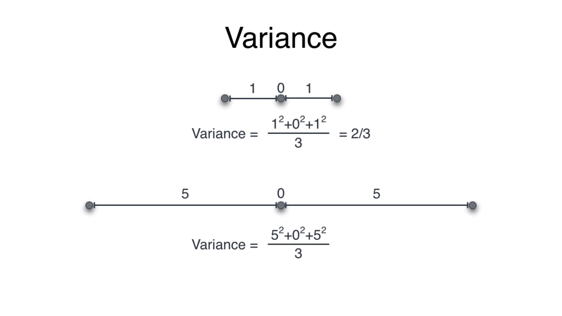
We take the square of each distance so we do not get any negative values!

我们采用每个距离的平方，因此不会得到任何负值！

For 2-dimensional dataset, just take the variance after projecting it on each axis (shown later).

对于二维数据集，只需将其投影在每个轴上即可(稍后显示)。

协方差 (Covariance)

In two and higher dimensional two very different datasets could have same variance, leading to misinterpretations of data. For example, both the datasets below have the same variance even though they are entirely different.

在二维和更高维中，两个非常不同的数据集可能具有相同的方差，从而导致对数据的误解。 例如，以下两个数据集尽管完全不同，但具有相同的方差。

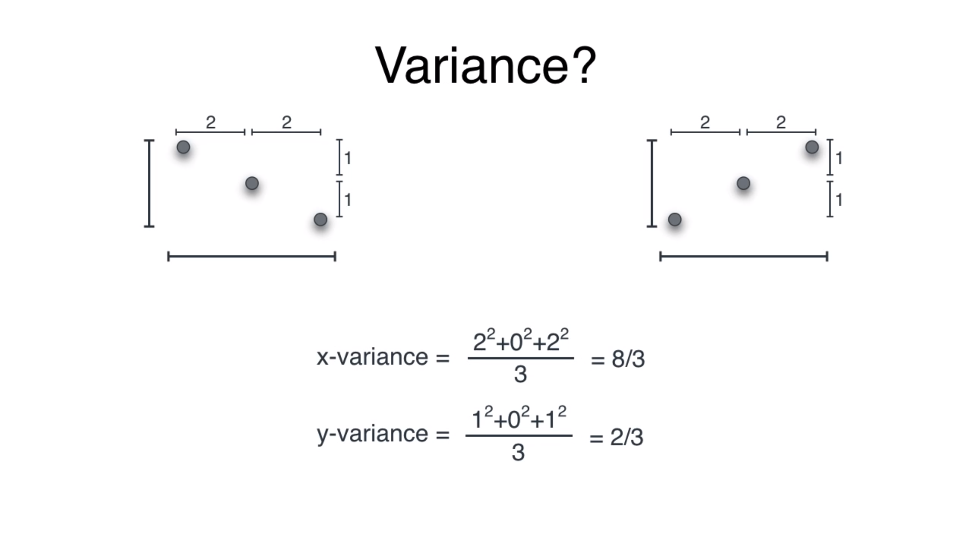
Notice that the variance is same for both entirely different datasets. Also note how x-variance and y-variance are calculated by projecting the data on each axis.

请注意，两个完全不同的数据集的方差相同。 还要注意如何通过将数据投影到每个轴上来计算x方差和y方差。

Covariance depicts the correlation of dataset. It is a quantity describing the variance as well as the direction of the spread. This will help us distinguish between the above two datasets.

协方差描述了数据集的相关性。 它是描述方差以及价差方向的数量。 这将有助于我们区分上述两个数据集。

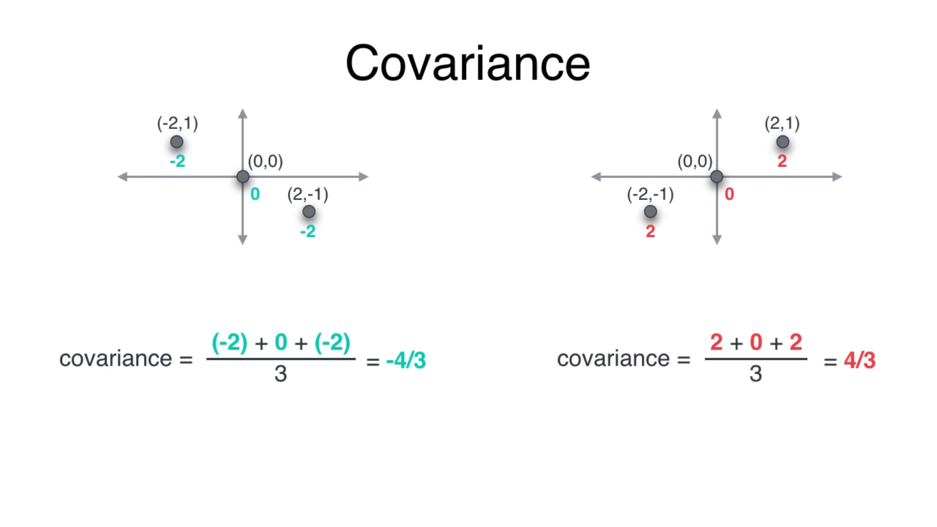
To get the covariance simply add the product of coordinates of each point. For example in red dataset. (-2, -1) results in 2 and so does (2, 1).

要获得协方差，只需添加每个点的坐标乘积 。 例如在红色数据集中。 (-2，-1)得出2，(2，1)也是如此。

The covariance matrix is a linear transformation that transforms given data into another shape. We will see that later. In 2D, this matrix is (2 x 2).

协方差矩阵是将给定数据转换为另一种形状的线性变换。 我们稍后会看到。 在2D模式下，此矩阵为(2 x 2)。

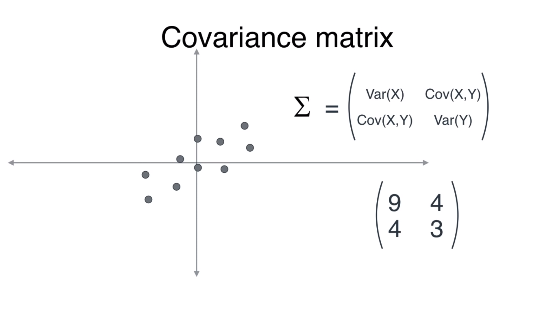
For the dataset in the example above, after inserting values, a rough estimate of the covariance matrix would be the one shown. To understand the use of this matrix we first need to understand linear transformations.

对于上面示例中的数据集，在插入值之后，将显示协方差矩阵的粗略估计。 要了解此矩阵的用法，我们首先需要了解线性变换。

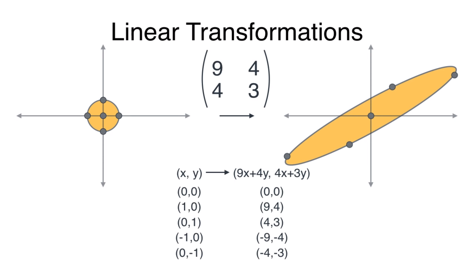
A linear transformation is a mapping that transforms any point in the 2D plane to another point in the same plane by using a transformation matrix.

线性变换是通过使用变换矩阵将2D平面中的任何点转换为同一平面中的另一个点的映射。

Back to our example, the covariance matrix is our transformation matrix. A unit circle would be transformed into an ellipse by the covariance matrix (using matrix multiplication) as shown below.

回到我们的示例，协方差矩阵是我们的变换矩阵。 如下所示，通过协方差矩阵(使用矩阵乘法)将单位圆转换为椭圆。

This transformation gives us two very special vectors — the eigenvectors.

这种转换为我们提供了两个非常特殊的向量- 特征向量。

These eigenvectors are special because they are not affected by the transformation (their direction remains the same), they are only increased in magnitude. Below are the two vectors in red and teal color.

这些特征向量是特殊的，因为它们不受变换的影响(它们的方向保持不变)，仅在幅度上有所增加。 以下是红色和蓝绿色的两个向量。

Speaking abstractly, these are the vectors on which we shall project our data, that would help us reduce the dimensions.

抽象地说，这些是我们将在其上投影数据的向量，这将有助于我们减小尺寸。

The question is: which eigenvector to choose?

问题是：选择哪个特征向量？

Let me tell you, you are an intelligent person if you chose the red one, because I myself had absolutely no clue!

让我告诉您，如果您选择红色，您就是一个聪明的人，因为我自己绝对不知道！

Red is the better choice because it would retain maximum variance of the original dataset, which means maximum information is retained.

红色是更好的选择，因为它将保留原始数据集的最大方差，这意味着将保留最大的信息。

Imagine you had picked the other eigenvector. Projecting the data would cause most of the points to overlap each other, and you will thus lose information. This is because the x-variance is greater than the y-variance.

假设您选择了另一个特征向量。 投影数据会导致大多数点相互重叠，因此您将丢失信息。 这是因为x方差大于y方差。

有趣的部分：代码！ (The interesting part: the code!)

We will apply the algorithm on word embeddings, which is a very high dimensional vector representation of, well, words. The TensorFlow visualization for 10,000 words in 200 dimensions is something like this:

我们将把算法应用于单词嵌入，它是单词的非常高维的向量表示。 TensorFlow可视化在200个维度中的10,000个单词如下所示：

source: http://projector.tensorflow.org/

来源： http ： //projector.tensorflow.org/

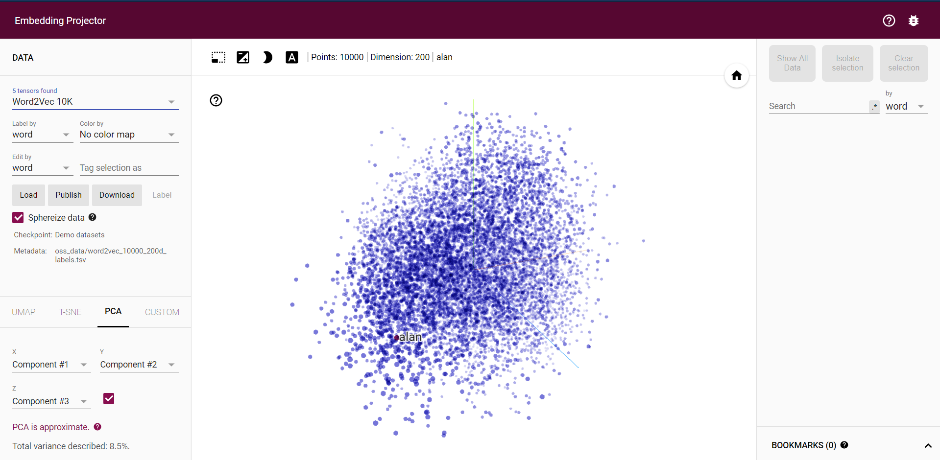
We will use a dataset with embeddings in 300 dimensions instead.

我们将使用在300个维度上嵌入的数据集。

How our dataset is arranged.

我们的数据集如何排列。

The process is as follows:

流程如下：

1. Demean the data (center it, so each feature has zero mean);
   对数据进行平均处理(将其居中，因此每个特征均值为零)；

def compute_pca(X, n_components=2):
    """
    Input:
        X: of dimension (m,n) where each row corresponds to a word vector
        n_components: Number of components you want to keep.
    Output:
        X_reduced: data transformed in 2 dims/columns + regenerated original data
    """    # mean center the data (axis=0 because taking mean along columns)
    X_demeaned = X - np.mean(X, axis=0, keepdims=True) # normalize each feature of dataset

2. Compute the covariance matrix;

2.计算协方差矩阵；

# calculate the covariance matrix, rowvar=False because our features are in columns, not rows
    covariance_matrix = np.cov(X_demeaned, rowvar=False)

3. Compute and sort the eigenvectors and eigenvalues from highest to lowest magnitude (eigenvalues), remember we need high eigenvalue eigenvectors so as to retain maximum variance (information) of our word embeddings.

3.计算特征向量和特征值从最高到最低的特征值(特征值)并进行排序，请记住，我们需要较高的特征值特征向量，以保留词嵌入的最大方差(信息)。

    # calculate eigenvectors & eigenvalues of the covariance matrix,           both are returned in ascending order
    eigen_vals, eigen_vecs = np.linalg.eigh(covariance_matrix)    # sort the eigen values (highest - lowest)
    eigen_vals_sorted = np.flip(eigen_vals)
    
    # sort eigenvectors (highest - lowest)
    eigen_vecs_sorted = np.flip(eigen_vecs, axis=1)

4. Select the n eigenvectors corresponding to the eigenvalues in descending order.

4.按降序选择与特征值相对应的n个特征向量。

    # select the first n eigenvectors (n is desired dimension
    # of rescaled data array, or dims_rescaled_data), each      eigenvector is a column in eigen_vecs matrix.    eigen_vecs_subset = eigen_vecs_sorted[:, :n_components]

5. Multiply this subset of eigenvectors by the demeaned data to get the transformed data!

5.将特征向量的这个子集乘以经过除法的数据，即可获得转换后的数据！

   # transform the data by multiplying the demeaned dataset with the    first n eigenvectors    X_reduced = np.dot(X_demeaned, eigen_vecs_subset)
    return X_reduced

让我们想象一下！ (Let’s visualize!)

Let’s try this algorithm on some data.

让我们对某些数据尝试这种算法。

words = ['oil', 'gas', 'happy', 'sad', 'city', 'town',
         'village', 'country', 'continent', 'petroleum', 'joyful'] #11 words# given a list of words and the embeddings, it returns a matrix with all the embeddings
X = get_vectors(word_embeddings, words)
X.shape # returns (11, 300)

Applying our algorithm to reduce from 300 dimensions to 2 dimensions!

应用我们的算法将尺寸从300维减少到2维！

# We have done the plotting for you. Just run this cell.
result = compute_pca(X, 2)
plt.figure(figsize=(12,8))
plt.scatter(result[:, 0], result[:, 1])
for i, word in enumerate(words):
    plt.annotate(word, xy=(result[i, 0] - 0.05, result[i, 1] + 0.1), )plt.show()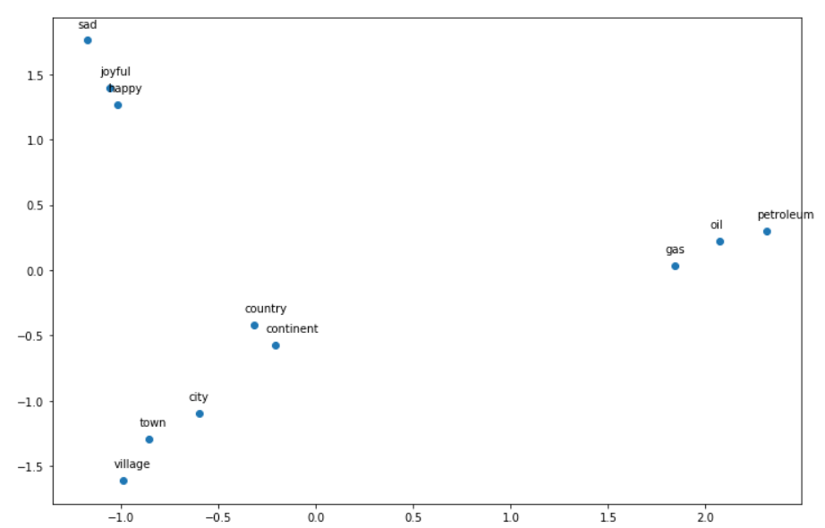

Takeaway: words that express emotions (sad, joyful, happy) are close to each other, town/village/city are close to each other as well, this is because they are highly related!

要点：表达情感(悲伤，快乐，快乐)的单词彼此接近，城镇/乡村/城市也彼此接近，这是因为它们之间有着密切的联系！

Now we have reduced 300 dimension embeddings to 2 dimension embeddings! That is why we can visualize it!

现在我们将300维嵌入减少为2维嵌入！ 这就是为什么我们可以将其可视化！

I hope I explained everything is a friendly and easy manner :)

我希望我解释的一切都是友好而轻松的方式:)

See you soon!

再见！

Note: All the slides shown in this article belong to a YouTube channel Luis Serrano. His video explaining PCA was amazing and here’s a link to his channel: https://www.youtube.com/channel/UCgBncpylJ1kiVaPyP-PZauQ

注意：本文中显示的所有幻灯片均属于YouTube频道Luis Serrano。 他的解释PCA的视频很棒，这是他的频道的链接： https : //www.youtube.com/channel/UCgBncpylJ1kiVaPyP-PZauQ

翻译自: https://medium.com/swlh/intuitive-explanation-for-principle-component-analysis-pca-from-scratch-157a1b162f1f

pca 主成分分析