如何在不重新平衡数据的情况下处理不平衡分类

In machine learning, when building a classification model with data having far more instances of one class than another, the initial default classifier is often unsatisfactory because it classifies almost every case as the majority class. Most of us are familiar with the fact that the ordinary classification accuracy score (% classified correctly) is not useful in the highly-imbalanced (skewed) case because it can trivially approach 100%, and it gives equal weight to false positives and false negatives. Many articles show you how to use oversampling (e.g. SMOTE) or sometimes class-based sample weighting to retrain the model, but this isn’t always necessary (and it also biases/distorts the numeric probability predictions of the model so that they become miscalibrated to the original and future data). Here we aim instead to show how much you can do without balancing the data or retraining the model, and how it gives you the flexibility to make any desired trade-off between false positives and false negatives.

在机器学习中，当使用一个类别比另一个类别具有更多实例的数据构建分类模型时，初始默认分类器通常不能令人满意，因为它几乎将每种情况都归类为多数类。 我们大多数人都熟悉以下事实：普通分类准确率得分(正确分类的百分比)在高度不平衡(偏斜)的情况下没有用，因为它可以微不足道地接近100％，并且对假阳性和假阴性给予同等的权重。 许多文章向您展示了如何使用过采样(例如SMOTE)或有时基于类的样本加权来重新训练模型，但这并不总是必要的(而且还会使模型的数字概率预测产生偏差/失真，从而使它们被错误校准)原始和将来的数据)。 在这里，我们的目的是显示在不平衡数据或重新训练模型的情况下您可以执行的操作，以及它如何使您灵活地在误报与误报之间做出所需的折衷。

We will use the credit card fraud identification data set from Kaggle to illustrate. Each row of the data set represents a credit card transaction, with the target variable Class==0 indicating a legitimate transaction and Class==1 indicating that the transaction turned out to be a fraud. There are 284,807 transactions, of which only 492 (0.173%) are frauds — very imbalanced indeed.

我们将使用来自Kaggle的信用卡欺诈识别数据集进行说明。 数据集的每一行代表一个信用卡交易，目标变量Class == 0表示合法交易，Class == 1表示该交易被证明是欺诈。 有284,807笔交易，其中只有492笔(0.173％)是欺诈-确实非常不平衡。

We will use a gradient boosting classifier because these often give good results. Specifically Scikit-Learn’s new HistGradientBoostingClassifier because it is much faster than their original GradientBoostingClassifier when the data set is relatively large like this one.

我们将使用梯度增强分类器，因为它们通常会产生良好的结果。 特别是Scikit-Learn的新HistGradientBoostingClassifier，因为当数据集相对较大时，它比其原始GradientBoostingClassifier快得多。

First let’s import some libraries and read in the data set.

首先，让我们导入一些库并读取数据集。

import numpy as np
import pandas as pd
from sklearn import model_selection, metrics
from sklearn.experimental import enable_hist_gradient_boosting
from sklearn.ensemble import HistGradientBoostingClassifier
df=pd.read_csv('creditcard.csv')
df.info()

V1 through V28 (from a principal components analysis) and the transaction Amount are the features, which are all numeric and there is no missing data. Because we are only using a tree-based classifier, we don’t need to standardize or normalize the features.

V1到V28(来自主成分分析)和交易额是要素，都是数字，没有丢失的数据。 因为我们仅使用基于树的分类器，所以不需要标准化或标准化功能。

We will now train the model after splitting the data into train and test sets. This took about half a minute on my laptop. We use the n_iter_no_change to stop the training early if the performance on a validation subset starts to deteriorate due to overfitting. I separately did a little bit of hyperparameter tuning to choose the learning_rate and max_leaf_nodes, but this is not the focus of the present article.

在将数据分为训练集和测试集后，我们现在将训练模型。 这在我的笔记本电脑上花费了大约半分钟。 如果验证子集的性能由于过度拟合而开始恶化，我们将使用n_iter_no_change尽早停止训练。 我分别做了一些超参数调整，以选择learning_rate和max_leaf_nodes，但这不是本文的重点。

Xtrain, Xtest, ytrain, ytest = model_selection.train_test_split(
        df.loc[:,'V1':'Amount'], df.Class,  stratify=df.Class, 
        test_size=0.3, random_state=42)
gbc=HistGradientBoostingClassifier(learning_rate=0.01, 
        max_iter=2000, max_leaf_nodes=6, validation_fraction=0.2, 
        n_iter_no_change=15, random_state=42).fit(Xtrain,ytrain)

Now we apply this model to the test data as the default hard-classifier, predicting 0 or 1 for each transaction. We are implicitly applying decision threshold 0.5 to the model’s probability prediction as a soft-classifier. When the probability prediction is over 0.5 we say “1” and when it is under 0.5 we say “0”.

现在，我们将此模型作为默认的硬分类器应用于测试数据，为每个事务预测0或1。 我们将决策阈值0.5作为软分类器隐式地应用于模型的概率预测。 当概率预测值大于0.5时，我们说“ 1”；当概率预测值小于0.5时，我们说“ 0”。

We also print the confusion matrix for the result, considering Class 1 (fraud) to be the “positive” class. The confusion matrix shows the number of True Negatives, False Positives, False Negatives, and True Positives. The normalized confusion matrix rates (e.g. FNR = False Negative Rate) are included as percentages in parentheses.

我们还将结果混淆矩阵打印出来，将第1类(欺诈)视为“正”类。 混淆矩阵显示“真阴性”，“假阳性”，“假阴性”和“真阳性”的数量。 归一化的混淆矩阵比率(例如FNR =假阴性比率)以百分比形式包含在括号中。

hardpredtst=gbc.predict(Xtest)
def conf_matrix(y,pred):
    ((tn, fp), (fn, tp)) = metrics.confusion_matrix(y, pred)
    ((tnr,fpr),(fnr,tpr))= metrics.confusion_matrix(y, pred, 
            normalize='true')
    return pd.DataFrame([[f'TN = {tn} (TNR = {tnr:1.2%})', 
                                f'FP = {fp} (FPR = {fpr:1.2%})'], 
                         [f'FN = {fn} (FNR = {fnr:1.2%})', 
                                f'TP = {tp} (TPR = {tpr:1.2%})']],
            index=['True 0(Legit)', 'True 1(Fraud)'], 
            columns=['Pred 0(Approve as Legit)', 
                            'Pred 1(Deny as Fraud)'])
conf_matrix(ytest,hardpredtst)

We see that the Recall for Class 1 (a.k.a. Sensitivity or True Positive Rate) is only 71.62%, so 28.38% of the true frauds are unfortunately approved as legitimate.

我们看到，第1类的召回率(即敏感性或真实肯定率)仅为71.62％，因此不幸的是，有28.38％的真实欺诈被批准为合法。

Especially with imbalanced data (or generally any time false positives and false negatives may have different consequences), it’s important not to limit ourselves to using the default implicit classification decision threshold of 0.5, as we did above by using “.predict()”. We want to improve the Recall of class 1 (the TPR) to reduce our fraud losses (reduce false negatives). To do this, we can reduce the threshold for which we say “Class 1” when we predict a probability above the threshold. This way we say “Class 1” for a wider range of predicted probabilities. Such strategies are known as threshold-moving.

尤其是在数据不平衡的情况下(或者通常在任何时候误报和误报可能会产生不同的后果)，重要的是不要将自己限制为使用默认的隐式分类决策阈值0.5，就像我们上面使用“ .predict()”所做的那样。 我们希望改善类别1(TPR)的召回率，以减少欺诈损失(减少误报)。 为此，当我们预测高于阈值的概率时，我们可以降低说“ Class 1”的阈值。 通过这种方式，我们说“类别1”可预测更大范围的概率。 这种策略称为阈值移动。

Ultimately it is a business decision to what extent we want to reduce these False Negatives since as a trade-off the number of False Positives (true legitimate transactions rejected as frauds) will inevitably increase as we adjust the threshold that we apply to the model’s probability prediction.

最终，这是一项业务决策，我们要在多大程度上减少这些误报率，因为作为一种折衷方案，随着我们调整适用于该模型概率的阈值，误报率(被拒绝为欺诈的真实合法交易)将不可避免地增加。预测。

To elucidate this trade-off and help us choose a threshold, we plot the False Positive Rate and False Negative Rate against the Threshold. This is a variant of the Receiver Operating Characteristic (ROC) curve, but emphasizing the threshold. (Note: if your classifier doesn’t have a predict_proba method, e.g. support vector classifiers, you can just as well use its decision_function method in its place.)

为了阐明这种权衡并帮助我们选择阈值，我们针对阈值绘制了误报率和误报率。 这是接收器工作特性(ROC)曲线的一种变体，但强调了阈值。 (注意：如果您的分类器没有predict_proba方法，例如支持向量分类器，则可以在其位置上使用其Decision_function方法。)

predtst=gbc.predict_proba(Xtest)[:,1]
fpr, tpr, thresholds = metrics.roc_curve(ytest, predtst)
dfplot=pd.DataFrame({'Threshold':thresholds, 
        'False Positive Rate':fpr, 
        'False Negative Rate': 1.-tpr})
ax=dfplot.plot(x='Threshold', y=['False Positive Rate',
        'False Negative Rate'], figsize=(10,6))
ax.plot([0.00035,0.00035],[0,0.1])
ax.set_xbound(0,0.0008); ax.set_ybound(0,0.3)

Although there exist some rules of thumb for choosing the optimal threshold, ultimately it depends on the cost to the business of false negatives vs. false positives. For example, looking at the plot above, we might choose to apply a threshold of 0.00035 (vertical green line has been added) as follows.

尽管存在一些选择最佳阈值的经验法则，但最终还是取决于假阴性与假阳性的业务成本。 例如，查看上面的图，我们可以选择如下应用阈值0.00035(已添加垂直绿线)。

hardpredtst_tuned_thresh = np.where(predtst >= 0.00035, 1, 0)
conf_matrix(ytest, hardpredtst_tuned_thresh)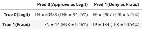

We have reduced our False Negative Rate to 9.46% (i.e. identified and denied 90.54% of our true frauds as our new Recall or True Positive Rate), while our False Positive Rate is 5.75% (i.e. still approved 94.25% of our legitimate transactions).

我们已将误报率降低至9.46％(即，将90.54％的真实欺诈识别并拒绝为新的召回率或真实积极率)，而我们的误报率为5.75％(即仍批准了我们合法交易的94.25％) 。

结论 (Conclusion)

Instead of naively applying a default threshold of 0.5, or immediately re-training using over-sampled or under-sampled or weighted classes, we can try using the original model (trained on the original “imbalanced” data set) and simply plot the trade-off between false positives and false negatives to choose a threshold that may produce a desirable business result.

我们可以尝试使用原始模型(在原始“不平衡”数据集上进行训练)来尝试绘制交易，而不是天真的应用默认阈值0.5或立即使用过采样或欠采样或加权类别进行重新训练。在误报和误报之间切换，以选择可能产生理想业务结果的阈值。

Please leave a response below if you have questions or comments (tap the speech bubble icon).

如果您有任何疑问或意见，请在下面留下答复(点击对话气泡图标)。

翻译自: https://towardsdatascience.com/how-to-deal-with-imbalanced-classification-without-re-balancing-the-data-8a3c02353fe3