浅谈对机器学习方法（决策树，SVM，knn最近邻，随机森林，朴素贝叶斯、逻辑回归）的理解以及用sklearn工具实现文本分类和回归方法...

一、决策树

 　　定下一个最初的质点，从该点出发、分叉。（由于最初质点有可能落在边界值上，此时有可能会出现过拟合的问题。

二、SVM

　　  svm是除深度学习在深度学习出现之前最好的分类算法了。它的特征如下：

　　（1）它既可应用于线性（回归问题）分类，也可应用于非线性分类;

　　（2）通过调节核函数参数的设置，可将数据集映射到多维平面上，对其细粒度化，从而使它的特征从二维变成多维，将在二维上线性不可分的问题转化为在多维上线性可　　　　  分的问题，最后再寻找一个最优切割平面（相当于在决策数基础上再寻找一个最优解），因此svm的分类效果是优于大多数的机器学习分类方法的。

　　（3）通过其它参数的设置，svm还可以防止过拟合的问题。

 推荐学习博客（哒哒师兄大大地推荐的喔~）：支持向量机通俗导论（理解SVM的三层境界）

三、随机森林

　　为了防止过拟合的问题，随机森林相当于多颗决策树。

 

四、knn最近邻

　　由于knn在每次寻找下一个离它最近的点时，都要将余下所有的点遍历一遍，因此其算法代价十分高。

 

五、朴素贝叶斯

要推事件A发生的概率下B发生的概率（其中事件A、B均可分解成多个事件），就可以通过求事件B发生的概率下事件A发生的概率，再通过贝叶斯定理计算即可算出结果。

 

六、逻辑回归

　　（离散型变量，二分类问题，只有两个值0和1）

 

本文主要参考了scikit-learn的官方网站 

用scikit-learn的基本分类方法（决策树、SVM、KNN）和集成方法（随机森林，Adaboost和GBRT）

1. 数据准备

关于分类,我们使用了Iris数据集,这个scikit-learn自带了. 
Iris数据集是常用的分类实验数据集，由Fisher, 1936收集整理。Iris也称鸢尾花卉数据集，是一类多重变量分析的数据集。数据集包含150个数据集，分为3类，每类50个数据，每个数据包含4个属性。可通过花萼长度，花萼宽度，花瓣长度，花瓣宽度4个属性预测鸢尾花卉属于（Setosa，Versicolour，Virginica）三个种类中的哪一类。

注意,Iris数据集给出的三种花是按照顺序来的,前50个是第0类,51-100是第1类,101~150是第二类,如果我们分训练集和测试集的时候要把顺序打乱 
这里我们引入一个两类shuffle的函数,它接收两个参数,分别是x和y,然后把x,y绑在一起shuffle.

 1 def shuffle_in_unison(a, b):
 2     assert len(a) == len(b)
 3     import numpy
 4     shuffled_a = numpy.empty(a.shape, dtype=a.dtype)
 5     shuffled_b = numpy.empty(b.shape, dtype=b.dtype)
 6     permutation = numpy.random.permutation(len(a))
 7     for old_index, new_index in enumerate(permutation):
 8         shuffled_a[new_index] = a[old_index]
 9         shuffled_b[new_index] = b[old_index]
10     return shuffled_a, shuffled_b

 

下面我们导入Iris数据并打乱它,然后分为100个训练集和50个测试集

 

1 from sklearn.datasets import load_iris
2 
3 iris = load_iris()
4 def load_data():
5     iris.data, iris.target = shuffle_in_unison(iris.data, iris.target)
6     x_train ,x_test = iris.data[:100],iris.data[100:]
7     y_train, y_test = iris.target[:100].reshape(-1,1),iris.target[100:].reshape(-1,1)
8     return x_train, y_train, x_test, y_test

 

2. 试验各种不同的方法

常用的分类方法一般有决策树, SVM, kNN, 朴素贝叶斯, 集成方法有随机森林,Adaboost和GBDT 
完整代码如下:

 1 from sklearn.datasets import load_iris
 2 
 3 iris = load_iris()
 4 
 5 def shuffle_in_unison(a, b):
 6     assert len(a) == len(b)
 7     import numpy
 8     shuffled_a = numpy.empty(a.shape, dtype=a.dtype)
 9     shuffled_b = numpy.empty(b.shape, dtype=b.dtype)
10     permutation = numpy.random.permutation(len(a))
11     for old_index, new_index in enumerate(permutation):
12         shuffled_a[new_index] = a[old_index]
13         shuffled_b[new_index] = b[old_index]
14     return shuffled_a, shuffled_b
15 
16 def load_data():
17     iris.data, iris.target = shuffle_in_unison(iris.data, iris.target)
18     x_train ,x_test = iris.data[:100],iris.data[100:]
19     y_train, y_test = iris.target[:100].reshape(-1,1),iris.target[100:].reshape(-1,1)
20     return x_train, y_train, x_test, y_test
21 
22 
23 from sklearn import tree, svm, naive_bayes,neighbors
24 from sklearn.ensemble import BaggingClassifier, AdaBoostClassifier, RandomForestClassifier, GradientBoostingClassifier
25 
26 
27 x_train, y_train, x_test, y_test = load_data()
28 
29 clfs = {'svm': svm.SVC(),\
30         'decision_tree':tree.DecisionTreeClassifier(),
31         'naive_gaussian': naive_bayes.GaussianNB(), \
32         'naive_mul':naive_bayes.MultinomialNB(),\
33         'K_neighbor' : neighbors.KNeighborsClassifier(),\
34         'bagging_knn' : BaggingClassifier(neighbors.KNeighborsClassifier(), max_samples=0.5,max_features=0.5), \
35         'bagging_tree': BaggingClassifier(tree.DecisionTreeClassifier(), max_samples=0.5,max_features=0.5),
36         'random_forest' : RandomForestClassifier(n_estimators=50),\
37         'adaboost':AdaBoostClassifier(n_estimators=50),\
38         'gradient_boost' : GradientBoostingClassifier(n_estimators=50, learning_rate=1.0,max_depth=1, random_state=0)
39         }
40 
41 def try_different_method(clf):
42     clf.fit(x_train,y_train.ravel())
43     score = clf.score(x_test,y_test.ravel())
44     print('the score is :', score)
45 
46 for clf_key in clfs.keys():
47     print('the classifier is :',clf_key)
48     clf = clfs[clf_key]
49     try_different_method(clf)

 

给出的结果如下:

 1 the classifier is : svm
 2 the score is : 0.94
 3 the classifier is : decision_tree
 4 the score is : 0.88
 5 the classifier is : naive_gaussian
 6 the score is : 0.96
 7 the classifier is : naive_mul
 8 the score is : 0.8
 9 the classifier is : K_neighbor
10 the score is : 0.94
11 the classifier is : gradient_boost
12 the score is : 0.88
13 the classifier is : adaboost
14 the score is : 0.62
15 the classifier is : bagging_tree
16 the score is : 0.94
17 the classifier is : bagging_knn
18 the score is : 0.94
19 the classifier is : random_forest
20 the score is : 0.92

 

 

 

 用scikit-learn的基本回归方法（线性、决策树、SVM、KNN）和集成方法（随机森林，Adaboost和GBRT）

前言：本教程主要使用了numpy的最最基本的功能，用于生成数据，matplotlib用于绘图，scikit-learn用于调用机器学习方法。如果你不熟悉他们（我也不熟悉）,没关系，看看numpy和matplotlib最简单的教程就够了。我们这个教程的程序不超过50行

1. 数据准备

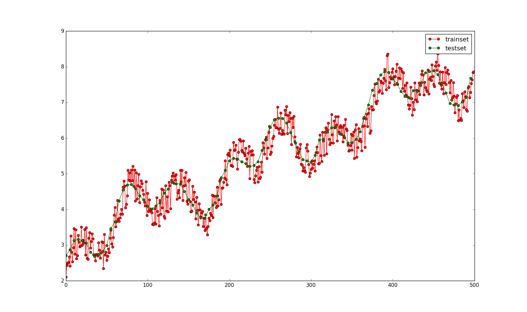
为了实验用，我自己写了一个二元函数，y=0.5*np.sin(x1)+ 0.5*np.cos(x2)+0.1*x1+3。其中x1的取值范围是0~50，x

 1 def f(x1, x2):
 2     y = 0.5 * np.sin(x1) + 0.5 * np.cos(x2)  + 0.1 * x1 + 3 
 3     return y
 4 
 5 def load_data():
 6     x1_train = np.linspace(0,50,500)
 7     x2_train = np.linspace(-10,10,500)
 8     data_train = np.array([[x1,x2,f(x1,x2) + (np.random.random(1)-0.5)] for x1,x2 in zip(x1_train, x2_train)])
 9     x1_test = np.linspace(0,50,100)+ 0.5 * np.random.random(100)
10     x2_test = np.linspace(-10,10,100) + 0.02 * np.random.random(100)
11     data_test = np.array([[x1,x2,f(x1,x2)] for x1,x2 in zip(x1_test, x2_test)])
12     return data_train, data_test

 

其中训练集（y上加有-0.5~0.5的随机噪声）和测试集（没有噪声）的图像如下： 

2. scikit-learn最简单的介绍。

scikit-learn非常简单，只需实例化一个算法对象，然后调用fit()函数就可以了，fit之后，就可以使用predict()函数来预测了，然后可以使用score(）函数来评估预测值和真实值的差异，函数返回一个得分。例如调用决策树的方法如下:

 1 In [6]: from sklearn.tree import DecisionTreeRegressor
 2 
 3 In [7]: clf = DecisionTreeRegressor()
 4 
 5 In [8]: clf.fit(x_train,y_train)
 6 Out[11]:
 7 DecisionTreeRegressor(criterion='mse', max_depth=None, max_features=None,
 8            max_leaf_nodes=None, min_samples_leaf=1, min_samples_split=2,
 9            min_weight_fraction_leaf=0.0, presort=False, random_state=None,
10            splitter='best')
11 In [15]: result = clf.predict(x_test)
12 
13 In [16]: clf.score(x_test,y_test)
14 Out[16]: 0.96352052312508396
15 
16 In [17]: result
17 Out[17]:
18 array([ 2.44996735,  2.79065744,  3.21866981,  3.20188779,  3.04219101,
19         2.60239551,  3.35783805,  2.40556647,  3.12082094,  2.79870458,
20         2.79049667,  3.62826131,  3.66788213,  4.07241195,  4.27444808,
21         4.75036169,  4.3854911 ,  4.52663074,  4.19299748,  4.42235821,
22         4.48263415,  4.16192621,  4.40477767,  3.76067775,  4.35353213,
23         4.6554961 ,  4.99228199,  4.29504731,  4.55211437,  5.08229167,

 

接下来，我们可以根据预测值和真值来画出一个图像。画图的代码如下：

 

1     plt.figure()
2     plt.plot(np.arange(len(result)), y_test,'go-',label='true value')
3     plt.plot(np.arange(len(result)),result,'ro-',label='predict value')
4     plt.title('score: %f'%score)
5     plt.legend()
6     plt.show()

 

然后图像会显示如下： 

3. 开始试验各种不同的回归方法

为了加快测试, 这里写了一个函数,函数接收不同的回归类的对象,然后它就会画出图像,并且给出得分. 
函数基本如下:

 1 def try_different_method(clf):
 2     clf.fit(x_train,y_train)
 3     score = clf.score(x_test, y_test)
 4     result = clf.predict(x_test)
 5     plt.figure()
 6     plt.plot(np.arange(len(result)), y_test,'go-',label='true value')
 7     plt.plot(np.arange(len(result)),result,'ro-',label='predict value')
 8     plt.title('score: %f'%score)
 9     plt.legend()
10     plt.show()

1 train, test = load_data()
2 x_train, y_train = train[:,:2], train[:,2] #数据前两列是x1,x2 第三列是y,这里的y有随机噪声
3 x_test ,y_test = test[:,:2], test[:,2] # 同上,不过这里的y没有噪声

3.1 常规回归方法

常规的回归方法有线性回归,决策树回归,SVM和k近邻(KNN)

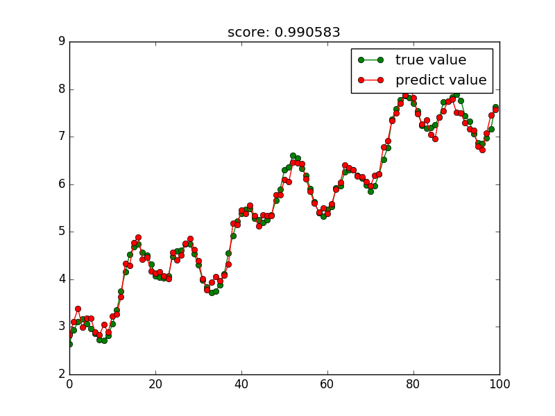
3.1.1 线性回归

1 In [4]: from sklearn import linear_model
2 
3 In [5]: linear_reg = linear_model.LinearRegression()
4 
5 In [6]: try_different_method(linar_reg)

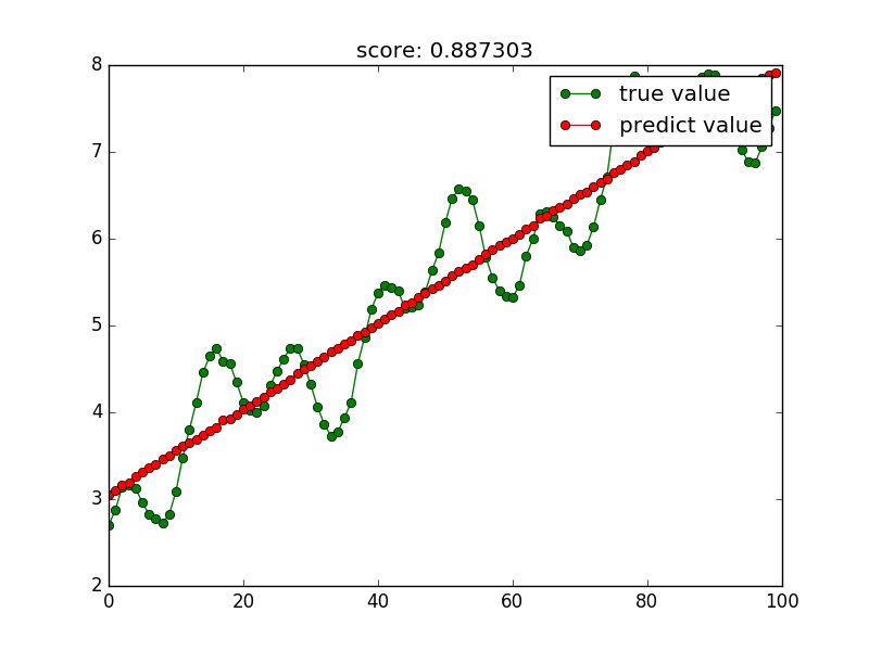
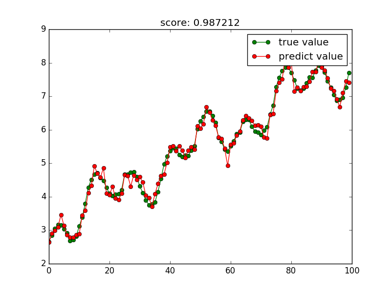
3.1.2数回归

1 from sklearn import tree
2 tree_reg = tree.DecisionTreeRegressor()
3 try_different_method(tree_reg)

 

然后决策树回归的图像就会显示出来: 

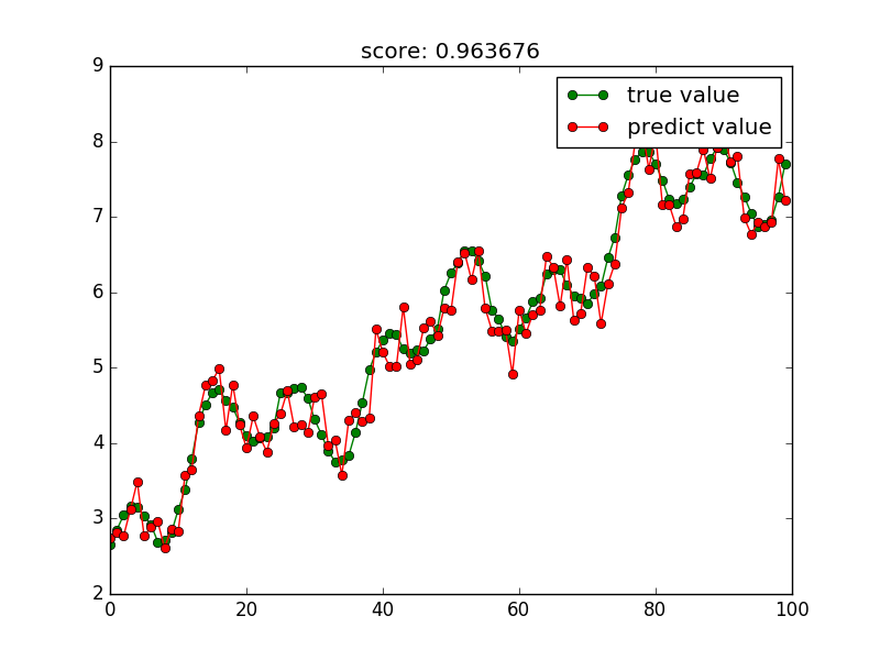
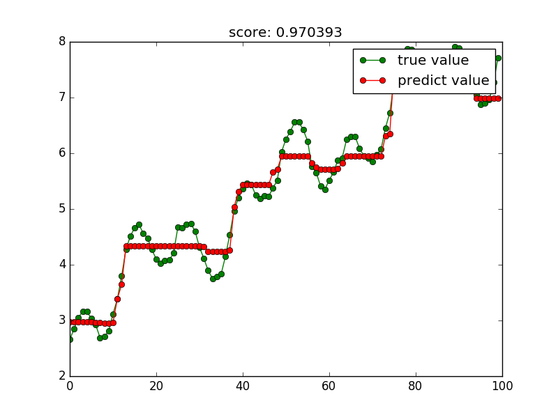
3.1.3 SVM回归

1 In [7]: from sklearn import svm
2 
3 In [8]: svr = svm.SVR()
4 
5 In [9]: try_different_method(svr)

结果图像如下: 

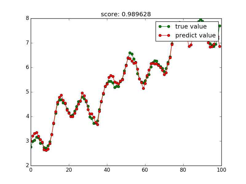
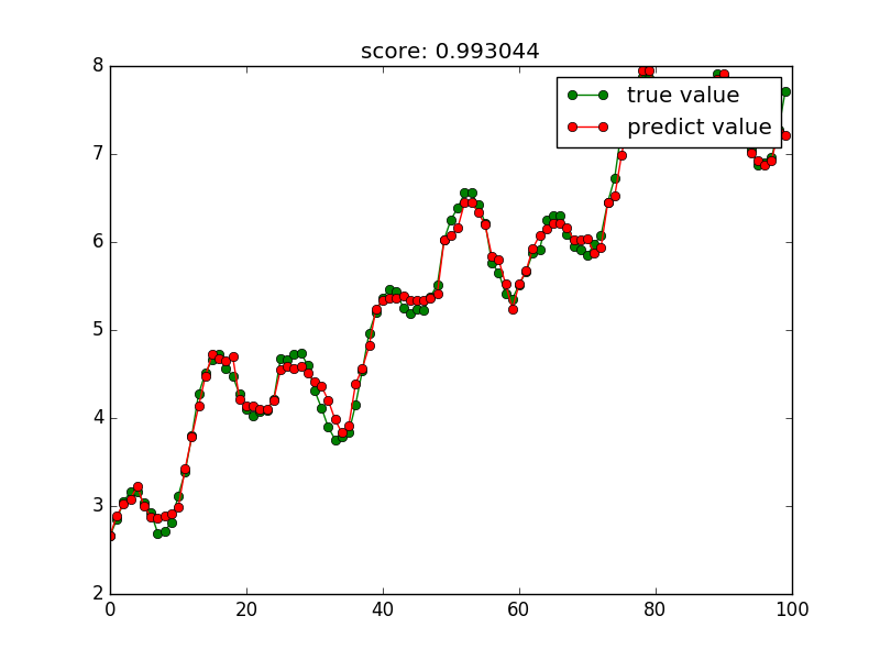
3.1.4 KNN

1 In [11]: from sklearn import neighbors
2 
3 In [12]: knn = neighbors.KNeighborsRegressor()
4 
5 In [13]: try_different_method(knn)

竟然KNN这个计算效能最差的算法效果最好 

3.2 集成方法(随机森林,adaboost, GBRT)

3.2.1随机森林

1 In [14]: from sklearn import ensemble
2 
3 In [16]: rf =ensemble.RandomForestRegressor(n_estimators=20)#这里使用20个决策树
4 
5 In [17]: try_different_method(rf)

3.2.2 Adaboost

1 In [18]: ada = ensemble.AdaBoostRegressor(n_estimators=50)
2 
3 In [19]: try_different_method(ada)

图像如下: 

3.2.3 GBRT

1 In [20]: gbrt = ensemble.GradientBoostingRegressor(n_estimators=100)
2 
3 In [21]: try_different_method(gbrt)

图像如下 

4. scikit-learn还有很多其他的方法,可以参考用户手册自行试验.

5.完整代码

我这里在pycharm写的代码,但是在pycharm里面不显示图形,所以可以把代码复制到ipython中,使用%paste方法复制代码片. 
然后参照上面的各个方法导入算法,使用try_different_mothod()函数画图. 
完整代码如下:

 1 import numpy as np
 2 import matplotlib.pyplot as plt
 3 
 4 def f(x1, x2):
 5     y = 0.5 * np.sin(x1) + 0.5 * np.cos(x2) + 3 + 0.1 * x1 
 6     return y
 7 
 8 def load_data():
 9     x1_train = np.linspace(0,50,500)
10     x2_train = np.linspace(-10,10,500)
11     data_train = np.array([[x1,x2,f(x1,x2) + (np.random.random(1)-0.5)] for x1,x2 in zip(x1_train, x2_train)])
12     x1_test = np.linspace(0,50,100)+ 0.5 * np.random.random(100)
13     x2_test = np.linspace(-10,10,100) + 0.02 * np.random.random(100)
14     data_test = np.array([[x1,x2,f(x1,x2)] for x1,x2 in zip(x1_test, x2_test)])
15     return data_train, data_test
16 
17 train, test = load_data()
18 x_train, y_train = train[:,:2], train[:,2] #数据前两列是x1,x2 第三列是y,这里的y有随机噪声
19 x_test ,y_test = test[:,:2], test[:,2] # 同上,不过这里的y没有噪声
20 
21 def try_different_method(clf):
22     clf.fit(x_train,y_train)
23     score = clf.score(x_test, y_test)
24     result = clf.predict(x_test)
25     plt.figure()
26     plt.plot(np.arange(len(result)), y_test,'go-',label='true value')
27     plt.plot(np.arange(len(result)),result,'ro-',label='predict value')
28     plt.title('score: %f'%score)
29     plt.legend()
30     plt.show()

 参考资料：

http://blog.csdn.net/u010900574/article/details/52666291

http://blog.csdn.net/u010900574/article/details/52669072?locationNum=5

 

转载于:https://www.cnblogs.com/flippedkiki/p/7209076.html