


自定义Matplotlib:https://matplotlib.org/tutorials/introductory/customizing.html#sphx-glr-tutorials-introductory-customizing-py
图像教程:https://matplotlib.org/tutorials/introductory/images.html#sphx-glr-tutorials-introductory-images-py
画廊:https://matplotlib.org/gallery.html
使用指南
matplotlib拥有广泛的代码库,大多数都可以通过一个相当简单的概念框架和一些重要知识来理解
绘图需要在一系列级别上进行操作。绘图包的目的是帮助尽可能轻松的可视化数据,并提供所有必要的控制。
因此matplotlib中所有内容都是按层次结构进行组织。顶部是matplotlib状态机环境。简单函数用于将绘图元素添加到当前图形的当前轴
层次结构下的是面向对象接口的第一级,其中pyplot仅用于少数功能,例如图形创建,并且用户显示创建并跟踪图形和轴对象。在此级别,用户使用pyplot来创建图形,并且通过这些图形,可以创建一个或多个轴对象。
对于GUI应用程序中嵌入matplotlib图标非常重要,所以一般都使用pyplot级别
import matplotlib.pyplot as plt
import numpy as np
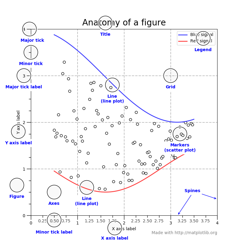
Figure
记录了所有子Axes,就是一些标签说明信息。一个数字可以有任意数量的Axes,但有用的应该至少有一个
fig = plt.figure()  # an empty figure with no axes
fig.suptitle('No axes on this figure') # Add a title so we know which it is fig, ax_lst = plt.subplots(2, 2) # a figure with a 2x2 grid of Axes
Axes
具有数据空间的图像区域。给定的图形可以包含许多轴,但给定的Axes对象只能在一个轴中Figure。轴包含两个Axis对象,负责数据限制。每个都有一个title(),一个x-label(),一个y-label()
Axis
负责设置图形限制并生成刻度线。刻度的位置有Locator对象确定,并且ticklabel字符串有a格式化Formatter。正确的组合Locator,并Formatter给出了刻度位置和标签非常精细的控制
绘制函数的输入类型
所有绘图功能都期望np.array或np.ma.masked_array作为输入。类似数组的类,例如pandas数据对象,np.martix可能会或可能不会按预期工作。最好np.array在绘图之前将这些转换为对象
a = pandas.DataFrame(np.random.rand(4,5), columns = list('abcde')) a_asndarray = a.values
Matplotlib, pyplot和pylab关系
Matplotlib是整个包,pyplot是一个模块并且pylab是一个安装在一起的模块。
pyplot为底层面向对象的绘图库提供状态机接口。状态机隐式地自动创建图形和轴以实现所需的图形
x = np.linspace(0, 2, 100)

plt.plot(x, x, label='linear')
plt.plot(x, x**2, label='quadratic')
plt.plot(x, x**3, label='cubic')

plt.xlabel('x label')
plt.ylabel('y label')

plt.title("Simple Plot")

plt.legend()

plt.show()
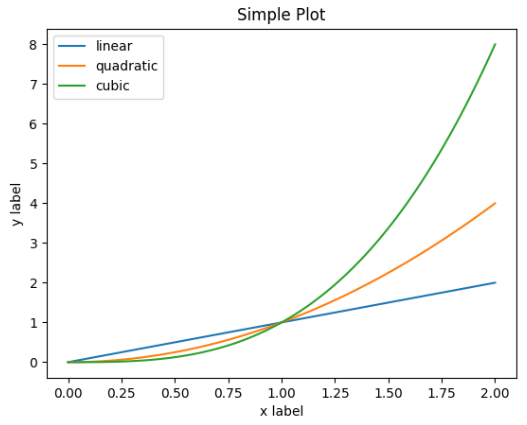
第一次调用plt.plot将自动创建必要的图形和轴以实现所需的图形。随后调用plt.plot重新使用当前轴并添加另一行。设置标题,图例和轴标签还会自动使用当前轴并设置标题,创建图例并分别标记轴
Pyplot简介
matplotlib.pyplot是一组命令样式函数,使matplotlib像MATLAB一样工作。每个pyplot函数都会对图形进行一些更改。
在matplotlib.pyplot函数调用中保留各种状态,以便跟踪当前图形和绘图区域等内容,并将绘图功能定向到当前轴。
import matplotlib.pyplot as plt
plt.plot([1, 2, 3, 4])
plt.ylabel('some numbers')
plt.show()
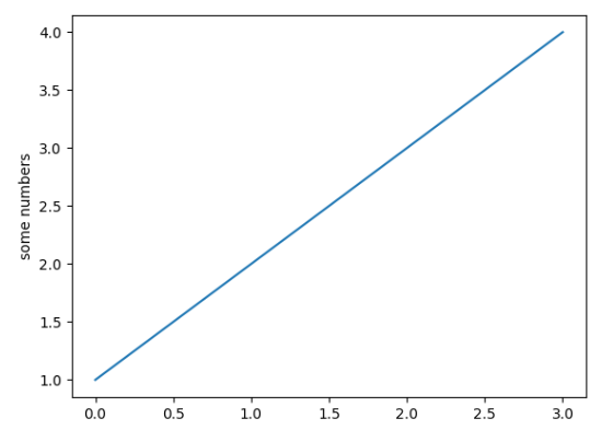
如果plot()命令提供单个列表或数组,matplotlib假定它是一系列y值,并自动为您生成x值。由于python范围以0开头,因此默认的x向量与y具有相同的长度,但从0开始。因此x数据为[0,1,2,3]
plot可以采取任意数量的论点,来设置x和y的关系。
plt.plot([1, 2, 3, 4], [1, 4, 9, 16])
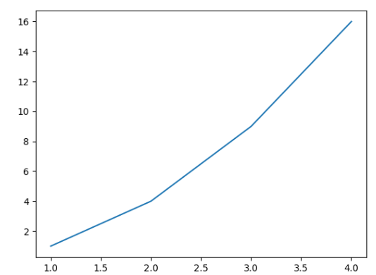
比如上面的图点就是1,1 - 2,4 - 3,9 - 4,16
格式化绘图样式
对于每对x,y的参数,都有一个可选的第三个参数,是格式字符串,用于指示绘图的颜色和线型。格式字符串的字母和符号来自MATLAB,将颜色字符串与线型字符串连接起来。默认格式字符串为蓝色实线。
如果要用红色圆圈绘制,可以如下修改
plt.plot([1, 2, 3, 4], [1, 4, 9, 16], 'ro')
plt.axis([0, 6, 0, 20])
plt.show()
axis:指定轴的大小值(xmin,xmax,ymin,ymax)
所有序列都在内部转换为numpy数组。比如下面使用数组绘制不同格式样式的行
import numpy as np
t = np.arange(0., 5., 0.2)
plt.plot(t, t, 'r--', t, t**2, 'bs', t, t**3, 'g^')
plt.show()

关键字字符绘图
某些情况下,可以使用numpy.recarray或pandas.DataFrame进行绘图操作
Matplotlib允许您使用data关键字参数提供此类对象。
data = {'a': np.arange(50),
        'c': np.random.randint(0, 50, 50),
        'd': np.random.randn(50)}
data['b'] = data['a'] + 10 * np.random.randn(50)
data['d'] = np.abs(data['d']) * 100

plt.scatter('a', 'b', c='c', s='d', data=data)
plt.xlabel('entry a')
plt.ylabel('entry b')
plt.show()
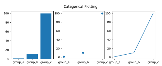
用分类变量绘图
可以使用分类变量创建绘图。允许将分类变量直接传递给许多绘图函数
names = ['group_a', 'group_b', 'group_c']
values = [1, 10, 100]

plt.figure(1, figsize=(9, 3))

plt.subplot(131)
plt.bar(names, values)
plt.subplot(132)
plt.scatter(names, values)
plt.subplot(133)
plt.plot(names, values)
plt.suptitle('Categorical Plotting')
plt.show()
控制线属性
行可以设置许多属性:线宽,短划线样式,抗锯齿等。看matplotlib.lines.Line2D。有几种方法可以设置线属性
使用关键字args
plt.plot(x, y, linewidth=2.0)
使用Line2D实例的setter方法。plot返回一个Line2D对象列表。假设我们只有一行,以便返回的列表长度为1.使用元组解包,获取该列表第一个元素
line, = plt.plot(x, y, '-') line.set_antialiased(False)
使用setp命令
使用MATLAB样式命令在行列表上设置多个属性。setp透明地使用对象列表或单个对象。可以使用python关键字参数或MATLAB样式的字符串
lines = plt.plot(x1, y1, x2, y2) # use keyword args plt.setp(lines, color='r', linewidth=2.0) # or MATLAB style string value pairs plt.setp(lines, 'color', 'r', 'linewidth', 2.0)
以下是可用的Line2D属性
属性:值类型
alpha:float
animated:[True | False]
antialiased or aa:[True | False]
clip_box:一个matplotlib.transform.Bbox实例
clip_on:[True | False]
clip_path:一个Path实例和一个Transform实例,一个Patch
color or c:任何matplotlib颜色
contains:命中测试功能
dash_capstyle:['butt' | 'round' | 'projecting']
dash_joinstyle:['miter' | 'round' | 'bevel']
dashes:点的开/关墨水序列
data:(np.array xdata, np.array ydata)
figure:一个matplotlib.figure.Figure实例
label:any string
linestyle or ls:[ '-' | '--' | '-.' | ':' | 'steps' | ...]
linewidth or lw:浮点数值
lod:[True | False]
marker:[ '+' | ',' | '.' | '1' | '2' | '3' | '4' ]
markeredgecolor or mec:any matplotlib color
markeredgewidth or mew:float value in points
markerfacecolor or mfc:any matplotlib color
markersize or ms:float
markevery:[ None | integer | (startind, stride) ]
picker:用于交互式线路选择
pickradius:行选择半径
solid_capstyle:['butt' | 'round' | 'projecting']
solid_joinstyle:['miter' | 'round' | 'bevel']
transform:一个matplotlib.transforms.Transform实例
visible:[True | False]
xdata:np.array
ydata:np.array
zorder:any number
要获取可设置的行属性列表,请setp()使用一行或多行作为参数调用该函数
lines = plt.plot([1, 2, 3])
plt.setp(lines)
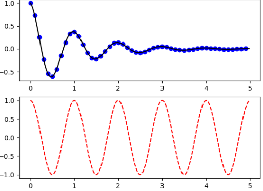
使用多个图形和轴
MATLAB,具有当前图形和当前轴的概念。所有绘图命令都适用于当前轴。gca() 返回当前轴(matplotlib.axes.Axes实例),gcf() 返回当前图形(matplotlib.figure.Figure实例)
def f(t):
    return np.exp(-t) * np.cos(2*np.pi*t)

t1 = np.arange(0.0, 5.0, 0.1)
t2 = np.arange(0.0, 5.0, 0.02)

plt.figure(1)
plt.subplot(211)
plt.plot(t1, f(t1), 'bo', t2, f(t2), 'k')

plt.subplot(212)
plt.plot(t2, np.cos(2*np.pi*t2), 'r--')
plt.show()
np.exp 指数函数通常特指以


figure此处的命令是可选的,因为figure(1)默认情况下将创建该命令,就像subplot(111)您不手动指定任何轴一样,默认情况下将创建该命令。subplot()命令指定其中范围从1到多少。
plt.subplot()关键参数有三个元素,分别代表行、列、当前激活的子图。比如plt.subplot(2,1,2),也可以去掉逗号写成plt.subplot(212)
可以创建任意数量的子图和轴,如果要手动放置轴,使用axes命令,该命令允许你指定所有值在小数(0到1)坐标中的位置。
可以使用figure具有增加的号,多个调用来创建多个数字。每个图形可以包含您心中所需的轴和子图
import matplotlib.pyplot as plt
plt.figure(1)                # the first figure
plt.subplot(211)             # the first subplot in the first figure
plt.plot([1, 2, 3])
plt.subplot(212)             # the second subplot in the first figure
plt.plot([4, 5, 6])


plt.figure(2)                # a second figure
plt.plot([4, 5, 6])          # creates a subplot(111) by default

plt.figure(1)                # figure 1 current; subplot(212) still current
plt.subplot(211)             # make subplot(211) in figure1 current
plt.title('Easy as 1, 2, 3') # subplot 211 title
可以使用clf 和 当前轴清除当前图形 cla。
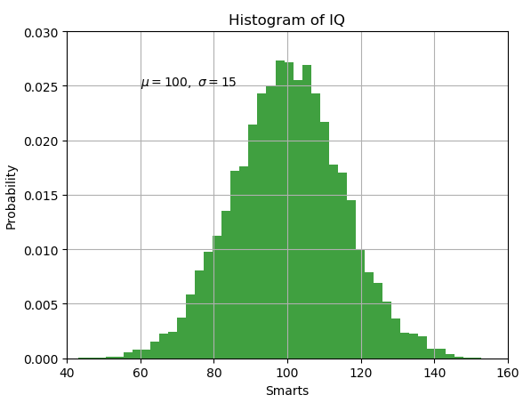
使用文本
text()命令可以用于在任意位置添加文本xlabel(),ylabel(),title()
mu, sigma = 100, 15
x = mu + sigma * np.random.randn(10000)

# the histogram of the data
n, bins, patches = plt.hist(x, 50, density=1, facecolor='g', alpha=0.75)


plt.xlabel('Smarts')
plt.ylabel('Probability')
plt.title('Histogram of IQ')
plt.text(60, .025, r'$\mu=100,\ \sigma=15$')
plt.axis([40, 160, 0, 0.03])
plt.grid(True)
plt.show()
所有text命令都返回一个matplotlib.text.Text实例。可以通过将关键字参数传递到文本函数或使用setp()以下内容来自定义属性
t = plt.xlabel('my data', fontsize=14, color='red')
文本中使用数学表达式
matplotlib在任何文本表达式中接受TeX方程表达式。要 在标题中编写表达式,可以编写由美元符号包围的TeX表达式
plt.title(r'$\sigma_i=15$')
不需要安装TeX,因为matplotlib附带了自己的TeX表达式解析器,布局引擎和字体。布局引擎是TeX中布局算法的直接改变,因此质量非常好
任何文本元素都可以使用数学文本。只要在引号前面加上r,并用美元符号$ 包围数学文本即可。
下面看一例子
plt.title(r'$\alpha > \beta$')

注意一定要放在两个$之间
下标和上标
要制作下标和上标,使用'_' 和 '^' 符号
r '$ \ alpha_i> \ beta_i $'
某些符号会自动将其子上标放在运算符下方和上方。例如写西格玛xi从0到无穷大
r '$ \ sum_ {i = 0} ^ \ infty x_i $'

分数,二项式和堆积数
分数,二项式和堆叠号码可以与被创建frac、binom、stackrel分别命令
r '$ \ frac {3} {4} \ binom {3} {4} \ stackrel {3} {4} $'

分数可以任意嵌套
r '$ \ frac {5 - \ frac {1} {x} } {4} $'
需要特别注意在分数周围放置括号。
r '$(\ frac {5 - \ frac {1} {x} } {4} )$'

r '$ \ left(\ frac {5 - \ frac {1} {x} } {4} \ right)$'

根号
使用\sqrt[]{}命令生成根号
r '$ \ sqrt {2} $'

可以在方括号内提供任何数据,基类必须是简单表达式,不能包含布局命令
r '$ \ sqrt [3] {x} $'

字体
数学符号的默认字体是斜体。要更改字体,将文本括在font命令中
r '$ s(t)= \ mathcal {A} \ mathrm {sin} (2 \ omega t)$'

许多罗马字体排版的常用函数名称都有快捷方式。上面的表达式可以写成如下
r '$ s(t)= \ mathcal {A} \ sin(2 \ omega t)$'

所有字体可用的选项是
命令:结果
\mathrm{Roman}:
\mathit{Italic}:
\mathtt{Typewriter}:
\mathcal{CALLIGRAPHY}:
\mathbb {blackboard}:
\mathrm {\mathbb{blackboard}}:
\mathfrak {Fraktur}:
\mathsf {sansserif}:
\mathrm {\mathsf{sansserif}}:
\mathcircled{circled}:
音节
重音命令可以在任何符号之前,在其上方添加重音。其中有一些长短形式
\acute a or \'a |  |
\bar a |  |
\breve a |  |
\ddot a or \"a |  |
\dot a or \.a |  |
\grave a or \`a |  |
\hat a or \^a |  |
\tilde a or \~a |  |
\vec a |  |
\overline{abc} |  |
此外,还有两种特殊的重音可以自动调整到下面符号的宽度
\widehat{xyz} |  |
\widetilde{xyz} |  |
在小写字母i 和 j添加重音时,应该用 \imath内容避免重叠到点上
r “$ \ hat i \ \ \ hat \ imath $”
符号
可以使用大量的TeX的符号
小写希腊语
\alpha
\beta
\chi
\delta\digamma\epsilon
\eta
\gamma
\iota\kappa\lambda
\mu
\nu
\omega
\phi
\pi
\psi
\rho
\sigma
\tau
\theta\upsilon\varepsilon\varkappa\varphi\varpi\varrho
\varsigma\vartheta
\xi
\zeta


大写希腊语
\Delta\Gamma\Lambda\Omega
\Phi
\Pi
\Psi\Sigma\Theta\Upsilon
\Xi\mho\nabla


希伯来语

\aleph
\beth
\daleth
\gimel
分隔符

/
[\Downarrow\Uparrow
\Vert\backslash\downarrow\langle
\lceil
\lfloor\llcorner\lrcorner
\rangle\rceil
\rfloor\ulcorner\uparrow\urcorner
\vert
\{
\|
\}
]
|


大符号
\bigcap\bigcup\bigodot\bigoplus\bigotimes\biguplus\bigvee\bigwedge\coprod
\int
\oint\prod
\sum


标准功能名称

\Pr\arccos\arcsin\arctan
\arg
\cos
\cosh
\cot
\coth
\csc
\deg
\det
\dim
\exp
\gcd
\hom
\inf
\ker
\lg
\lim\liminf\limsup
\ln
\log
\max
\min
\sec
\sin
\sinh
\sup
\tan
\tanh


二元运算和关系符号

\Bumpeq
\Cap
\Cup
\Doteq
\Join
\Subset
\Supset
\Vdash
\Vvdash
\approx
\approxeq
\ast
\asymp
\backepsilon
\backsim
\backsimeq
\barwedge
\because
\between
\bigcirc\bigtriangledown\bigtriangleup\blacktriangleleft\blacktriangleright
\bot
\bowtie
\boxdot
\boxminus
\boxplus
\boxtimes
\bullet
\bumpeq
\cap
\cdot
\circ
\circeq
\coloneq
\cong
\cup\curlyeqprec
\curlyeqsucc
\curlyvee
\curlywedge
\dag
\dashv
\ddag
\diamond
\div\divideontimes
\doteq
\doteqdot
\dotplus
\doublebarwedge
\eqcirc
\eqcolon
\eqsim
\eqslantgtr\eqslantless
\equiv
\fallingdotseq

\frown
\geq
\geqq
\geqslant
\gg
\ggg
\gnapprox
\gneqq
\gnsim
\gtrapprox
\gtrdot
\gtreqless
\gtreqqless
\gtrless
\gtrsim
\in
\intercal\leftthreetimes
\leq
\leqq
\leqslant
\lessapprox
\lessdot
\lesseqgtr
\lesseqqgtr
\lessgtr
\lesssim
\ll
\lll
\lnapprox
\lneqq
\lnsim
\ltimes
\mid
\models
\mp
\nVDash
\nVdash
\napprox
\ncong
\ne
\neq\neq
\nequiv
\ngeq
\ngtr
\ni
\nleq
\nless
\nmid
\notin
\nparallel
\nprec
\nsim
\nsubset
\nsubseteq
\nsucc
\nsupset
\nsupseteq\ntriangleleft
\ntrianglelefteq\ntriangleright\ntrianglerighteq
\nvDash
\nvdash
\odot
\ominus
\oplus
\oslash
\otimes
\parallel
\perp
\pitchfork
\pm
\prec
\precapprox
\preccurlyeq
\preceq
\precnapprox
\precnsim
\precsim
\propto\rightthreetimes
\risingdotseq
\rtimes
\sim
\simeq
\slash
\smile
\sqcap
\sqcup
\sqsubset\sqsubset
\sqsubseteq
\sqsupset\sqsupset
\sqsupseteq
\star
\subset
\subseteq
\subseteqq
\subsetneq
\subsetneqq
\succ
\succapprox
\succcurlyeq
\succeq
\succnapprox
\succnsim
\succsim
\supset
\supseteq
\supseteqq
\supsetneq
\supsetneqq
\therefore
\times
\top
\triangleleft\trianglelefteq

\triangleq
\triangleright\trianglerighteq
\uplus
\vDash
\varpropto\vartriangleleft\vartriangleright
\vdash
\vee
\veebar
\wedge
\wr


箭头符号

\Downarrow
\Leftarrow
\Leftrightarrow
\Lleftarrow
\Longleftarrow
\Longleftrightarrow
\Longrightarrow
\Lsh
\Nearrow
\Nwarrow
\Rightarrow
\Rrightarrow
\Rsh
\Searrow
\Swarrow
\Uparrow
\Updownarrow
\circlearrowleft
\circlearrowright
\curvearrowleft
\curvearrowright
\dashleftarrow
\dashrightarrow
\downarrow
\downdownarrows
\downharpoonleft
\downharpoonright
\hookleftarrow
\hookrightarrow
\leadsto
\leftarrow
\leftarrowtail
\leftharpoondown
\leftharpoonup
\leftleftarrows
\leftrightarrow
\leftrightarrows
\leftrightharpoons
\leftrightsquigarrow
\leftsquigarrow

\longleftarrow
\longleftrightarrow
\longmapsto
\longrightarrow
\looparrowleft
\looparrowright
\mapsto
\multimap
\nLeftarrow
\nLeftrightarrow
\nRightarrow
\nearrow
\nleftarrow
\nleftrightarrow
\nrightarrow
\nwarrow
\rightarrow
\rightarrowtail
\rightharpoondown
\rightharpoonup
\rightleftarrows\rightleftarrows
\rightleftharpoons\rightleftharpoons
\rightrightarrows\rightrightarrows
\rightsquigarrow
\searrow
\swarrow
\to
\twoheadleftarrow
\twoheadrightarrow
\uparrow
\updownarrow\updownarrow
\upharpoonleft
\upharpoonright
\upuparrows
杂项符号

\$
\AA
\Finv
\Game
\Im
\P
\Re
\S
\angle
\backprime
\bigstar\blacksquare\blacktriangle\blacktriangledown
\cdots
\checkmark
\circledR
\circledS
\clubsuit
\complement
\copyright
\ddots
\diamondsuit
\ell
\emptyset
\eth
\exists
\flat
\forall
\hbar
\heartsuit
\hslash
\iiint
\iint\iint
\imath
\infty
\jmath
\ldots\measuredangle
\natural
\neg
\nexists
\oiiint
\partial
\prime
\sharp
\spadesuit\sphericalangle
\ss\triangledown
\varnothing
\vartriangle
\vdots
\wp
\yen


示例
这是一个示例,说明了上下文中的许多这些功能。
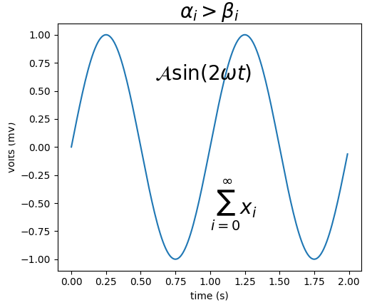
import numpy as np
import matplotlib.pyplot as plt
t = np.arange(0.0, 2.0, 0.01)
s = np.sin(2*np.pi*t)

plt.plot(t,s)
plt.title(r'$\alpha_i > \beta_i$', fontsize=20)
plt.text(1, -0.6, r'$\sum_{i=0}^\infty x_i$', fontsize=20)
plt.text(0.6, 0.6, r'$\mathcal{A}\mathrm{sin}(2 \omega t)$',
         fontsize=20)
plt.xlabel('time (s)')
plt.ylabel('volts (mV)')
plt.show()
注释文本
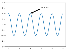
text 上面基本命令的使用将文本放在Axes上的任意位置。文本的常见用途是注释绘图的某些功能,并且该annotate() 方法提供帮助功能义使注释变得更容易
ax = plt.subplot(111)

t = np.arange(0.0, 5.0, 0.01)
s = np.cos(2*np.pi*t)
line, = plt.plot(t, s, lw=2)

plt.annotate('local max', xy=(2, 1), xytext=(3, 1.5),
             arrowprops=dict(facecolor='black', shrink=0.05),)

plt.ylim(-2, 2)
plt.show()
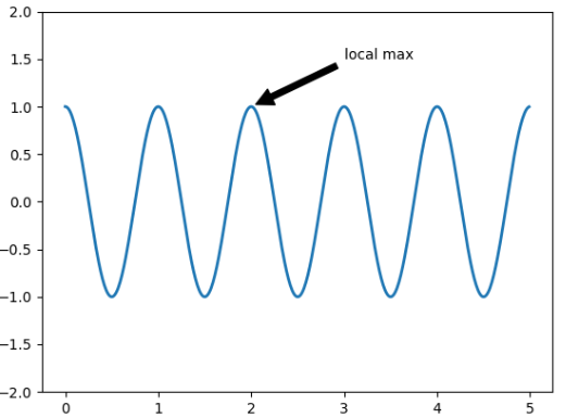
xy(箭头提示)和xytext位置都在数据坐标中。可以选择各种其他坐标系
注释
使用Matplotlib注释文本
基本的使用text() 将文本放在Axes上的任意位置。文本的常见用例是注释绘图的某些功能,并且该annotate() 方法提供帮助功能以使注释变得容易。
在注释中,有两点需要考虑:注释的位置由参数xy和文本的位置xytext表示。这两个参数都是(x,y)元组
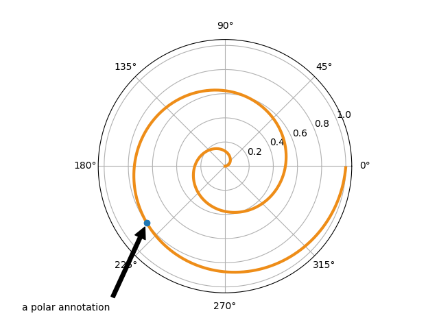
在上面的示例中,xy箭头是和xytext位置都在数据坐标中。可以选择各种其他坐标系,可以指定xy和xytext使用以下字符串之一的坐标系xycoords和textcoords默认为data
论据:坐标系
'figure points':从图的左下角开始的点
'figure pixels':图左下角的像素
'figure fraction':0,0是图的左下角,1,1是右上角
'axes points':从轴的左下角开始的点
'axes pixels':轴左下角的像素
'axes fraction':0,0位于轴的左下方,1,1位于右上方
'data':使用轴数据坐标系
要将文本坐标放在小数轴坐标中,可以执行以下操作
ax.annotate('local max', xy=(3, 1), xycoords='data', xytext=(0.8, 0.95), textcoords='axes fraction', arrowprops=dict(facecolor='black', shrink=0.05), horizontalalignment='right', verticalalignment='top', )
对于物理坐标系(点或像素),原点是图形的左下角
通过在可选关键字参数中提供箭头属性字典,可以启用文本到注释点的箭头绘制arrowprops
arrowprops 键:描述
width:点的箭头宽度
frac:头部占据的箭头长度的分数
headwidth:箭头底部的宽度以磅为单位
shrink:移动尖端并将基数与注释点和文本相差一些
**kwargs:任何关键matplotlib.patches.Polygon,例如,facecolor
在下面的示例中,xy点位于本机坐标中(xycoords默认为"data")。示例中文本放在小数字坐标系中。matplotlib.text.Text 关键字args喜欢horizontalalignment,verticalcalignment并fontsize传递annotate给Text示例
文本注释
text() pyplot模块中的函数(或Axes类的文本方法)采用bbox关键字参数,并且在给定时,将绘制文本周围的框
bbox_props = dict(boxstyle="rarrow,pad=0.3", fc="cyan", ec="b", lw=2) t = ax.text(0, 0, "Direction", ha="center", va="center", rotation=45, size=15, bbox=bbox_props)
可以通过以下方式访问与文本关联的修补程序对象
bb = t.get_bbox_patch()
返回值是FancyBboxPatch的一个实例,可以像往常一样访问和修改像facecolor,edgenwith等补丁属性。要更改框的形状,使用set_boxstyle方法
bb.set_boxstyle("rarrow", pad=0.6)
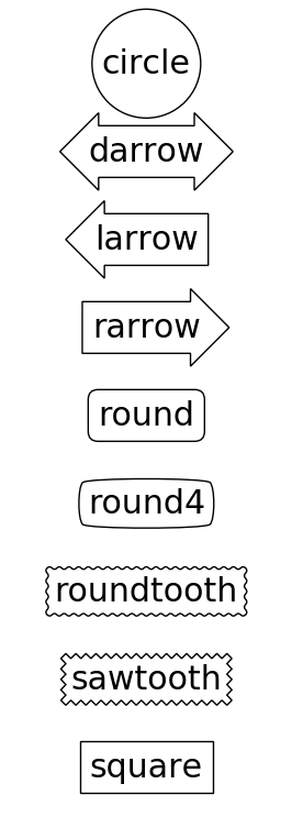
参数是框样式的名称,其属性为关键字参数。目前实现了以下框样式
Class:Name:Attrs
Circle:circle:pad=0.3
DArrow:darrow:pad=0.3
LArrow:larrow:pad=0.3
RArrow:rarrow:pad=0.3
Round:round:pad=0.3,rounding_size=None
Round4:round4:pad=0.3,rounding_size=None
Roundtooth:roundtooth:pad=0.3,tooth_size=None
Sawtooth:sawtooth:pad=0.3,tooth_size=None
Square:square:pad=0.3
请注意,可以使用分隔逗号在样式名称中指定属性参数
bb.set_boxstyle("rarrow,pad=0.6")
箭头注释
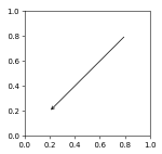
annotate() pyplot模块中的函数用于绘制连接图上两点的箭头
ax.annotate("Annotation", xy=(x1, y1), xycoords='data', xytext=(x2, y2), textcoords='offset points', )
在诠释一个点xy在给定的坐标为(xycoords),在文xytext中给出textcoords。通常,注释点在数据坐标中指定,而注释文本在偏移点中指定。
可以通过指定arrowprops参数来选择性地绘制连接两个点(xy和xytext)的箭头。要绘制箭头,请使用空字符串作为第一个参数
ax.annotate("", xy=(0.2, 0.2), xycoords='data', xytext=(0.8, 0.8), textcoords='data', arrowprops=dict(arrowstyle="->", connectionstyle="arc3"), )
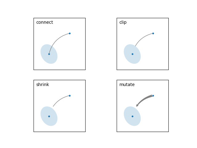
箭头绘制需要几个步骤
1.创建两点之间的连接路径。connectionstyle键值控制
2.如果给出乐力补丁对象patchA和patchB,则剪切路径以避免补丁
3.给定数量的像素进一步缩小路径
4.路径转换为箭头补丁,arrowstyle键值控制
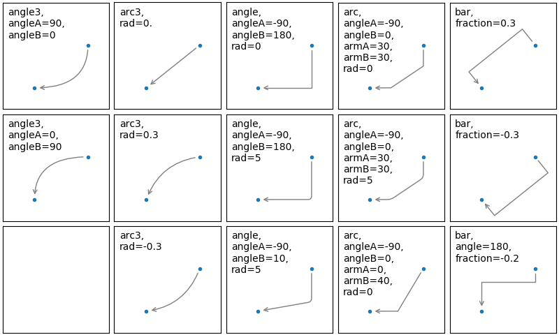
两点之间的乱接路径的创建由connectionstyle键控制,并且可以使用以下样式
Name:Attrs
angle:angleA=90,angleB=0,rad=0.0
angle3:angleA=90,angleB=0
arc:angleA=0,angleB=0,armA=None,armB=None,rad=0.0
arc3:rad=0.0
bar:armA=0.0,armB=0.0,fraction=0.3,angle=None
angle3和arc3 表示结果路径是二次样条线段。当链接路径是二次样条时,才能使用某些箭头样式选项
然后根据给定的链接路径变为箭头补丁arrowstyle
Name:Attrs
-:None
->:head_length=0.4,head_width=0.2
-[:widthB=1.0,lengthB=0.2,angleB=None
|-|:widthA=1.0,widthB=1.0
-|>:head_length=0.4,head_width=0.2
<-:head_length=0.4,head_width=0.2
<->:head_length=0.4,head_width=0.2
<|-:head_length=0.4,head_width=0.2
<|-|>:head_length=0.4,head_width=0.2
fancy:head_length=0.4,head_width=0.4,tail_width=0.4
simple:head_length=0.5,head_width=0.5,tail_width=0.2
wedge:tail_width=0.3,shrink_factor=0.5
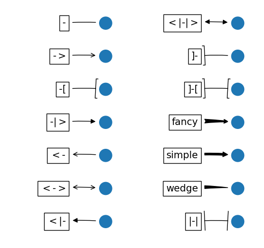
某些箭头样式仅适用于生成二次样条线段的连接样式。他们是fancy,simple,wedge。对于这些箭头样式,必须使用angle3或arc3链接样式
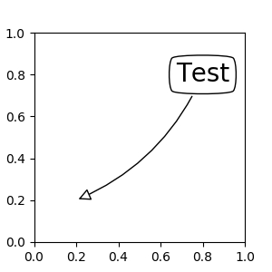
如果给出了注释字符串,则默认情况下patchA设置为文本bbox补丁
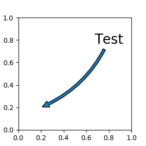
与在text命令中一样,可以使用bbox参数绘制文本周围的框
将Artists放置在Axes的锚定位置
有些Artists可以防止在Axes的锚定位置。可以使用OffsetBox类创建
mpl_toolkits.axes_grid1,anchored_artists可以使用一些预定义的类matplotlib.offsetbox
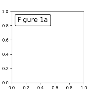
from matplotlib.offsetbox import AnchoredText
at = AnchoredText("Figure 1a", prop=dict(size=8), frameon=True, loc=2, ) at.patch.set_boxstyle("round,pad=0.,rounding_size=0.2") ax.add_artist(at)
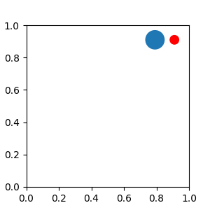
一个简单的应用是在Artists的大小在创作期间以像素大小知道的时候。如果要绘制固定大小为20*20的圆,则可以使用AnchoredDrawingArea,使用绘图区域的大小创建实例,并且可以将任意Artists添加到绘图区域。添加到绘图区域的艺术家的范围与绘图区域本身的位置无关。只有初始尺寸很重要。
from mpl_toolkits.axes_grid1.anchored_artists import AnchoredDrawingArea

ada = AnchoredDrawingArea(20, 20, 0, 0, loc=1, pad=0., frameon=False) p1 = Circle((10, 10), 10) ada.drawing_area.add_artist(p1) p2 = Circle((30, 10), 5, fc="r") ada.drawing_area.add_artist(p2)
添加到绘图区域的Artists不应该具有变换集,并且这些Artists的尺寸被解释为像素坐标,即上例中的圆的半径分别是10像素和5像素
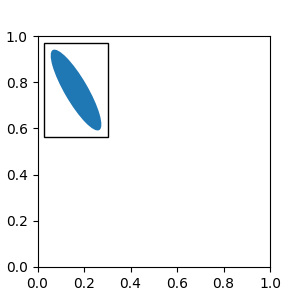
如果希望Artists使用数据坐标进行缩放,可以使用AnchoredAuxTransformBox课程。类似于除了Artists的范围是在绘图时间内根据指定的变换确定的。
from mpl_toolkits.axes_grid1.anchored_artists import AnchoredAuxTransformBox

box = AnchoredAuxTransformBox(ax.transData, loc=2) el = Ellipse((0,0), width=0.1, height=0.4, angle=30) # in data coordinates! box.drawing_area.add_artist(el)
例子中椭圆在数据坐标中的宽度和高度对应于0.1和0.4,并且当轴的视图极限发生变化时将自动缩放
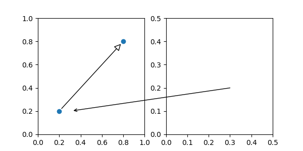
使用ConnectionPatch
ConnectionPatch就像没有文本的注释。大多数情况建议使用注释功能,但是想要链接不同轴上的点时,ConnectionPatch非常有用
from matplotlib.patches import ConnectionPatch
xy = (0.2, 0.2) con = ConnectionPatch(xyA=xy, xyB=xy, coordsA="data", coordsB="data", axesA=ax1, axesB=ax2) ax2.add_artist(con)
上面代码将数据坐标中的ax1点xy链接到数据坐标中的点xy ax2.这是一个简单的例子
虽然可以将ConnectionPatch实例添加到任何轴,但您可能希望将其添加到最新绘图顺序的轴,以防止其他轴重叠。
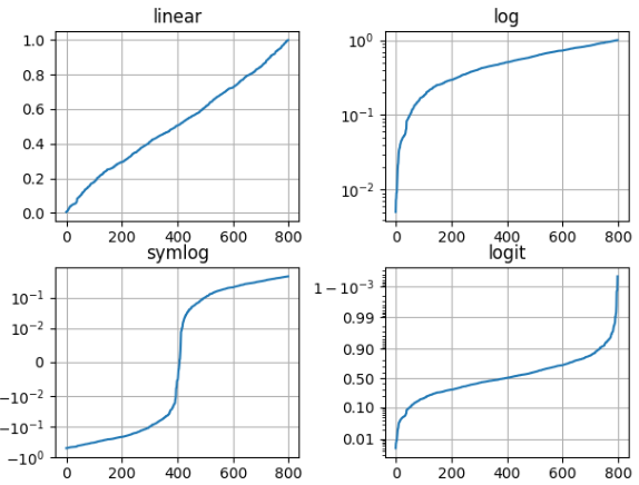
对数和其他非线性轴
matplotlib.pyplot不仅支持线性轴刻度,还支持对数和logit刻度。如果数据跨越许多数量级,则通常使用这种方法
from matplotlib.ticker import NullFormatter  # useful for `logit` scale

# Fixing random state for reproducibility
np.random.seed(19680801)

# make up some data in the interval ]0, 1[
y = np.random.normal(loc=0.5, scale=0.4, size=1000)
y = y[(y > 0) & (y < 1)]
y.sort()
x = np.arange(len(y))

# plot with various axes scales
plt.figure(1)

# linear
plt.subplot(221)
plt.plot(x, y)
plt.yscale('linear')
plt.title('linear')
plt.grid(True)


# log
plt.subplot(222)
plt.plot(x, y)
plt.yscale('log')
plt.title('log')
plt.grid(True)


# symmetric log
plt.subplot(223)
plt.plot(x, y - y.mean())
plt.yscale('symlog', linthreshy=0.01)
plt.title('symlog')
plt.grid(True)

# logit
plt.subplot(224)
plt.plot(x, y)
plt.yscale('logit')
plt.title('logit')
plt.grid(True)
# Format the minor tick labels of the y-axis into empty strings with
# `NullFormatter`, to avoid cumbering the axis with too many labels.
plt.gca().yaxis.set_minor_formatter(NullFormatter())
# Adjust the subplot layout, because the logit one may take more space
# than usual, due to y-tick labels like "1 - 10^{-3}"
plt.subplots_adjust(top=0.92, bottom=0.08, left=0.10, right=0.95, hspace=0.25,
                    wspace=0.35)

plt.show()
https://matplotlib.org/tutorials/introductory/pyplot.html


 527
527


 被折叠的 条评论
为什么被折叠?
被折叠的 条评论
为什么被折叠?
 到【灌水乐园】发言


