梯度下降

梯度下降法

在使用梯度下降法前，最好进行数据归一化

 

1. 不是一个机器学习算法
2. 是一种基于搜索的最优化方法
3. 作用：最小化损失函数
4. 梯度上升法，最大化一个效用函数

 

1. η称为学习率
2. η的值影响获得最优解的速度
3. η取值不合适甚至得不到最优解
4. η是梯度下降法的一个超参数

 

优势

 

特征越多的情况下，梯度下降相比于正规方程所耗时间更短，优势就体现出来了。

 

问题：存在多个极值点的情况？

 

1. 多次运行，随机化初始点
2. 梯度下降法的初始点也是一个超参数

 

tensorflow梯度下降实现多元线性回归

import tensorflow as tf
import numpy as np
import matplotlib.pyplot as plt
​
from sklearn import datasets
from sklearn.model_selection import train_test_split
from sklearn.linear_model import LinearRegression
from sklearn.preprocessing import StandardScaler
from sklearn.metrics import r2_score
 

# 加载数据
boston = datasets.load_boston()
x = boston.data
y = boston.target
​
trainX,testX,trainY,testY = train_test_split(x,y)
trainY = np.reshape(trainY,(-1,1))
# 数据归一化
standardScaler = StandardScaler()
standardScaler.fit(trainX)
trainX = standardScaler.transform(trainX)
testX = standardScaler.transform(testX)
print(trainX.shape)
print(trainY.shape)
 
>>>(379, 13)
>>>(379, 1)

 
# tensorflow
data_input = tf.placeholder(dtype=tf.float32,shape=(None,13))
label_input = tf.placeholder(dtype=tf.float32,shape=(None,1))
​
a = tf.Variable(tf.ones(shape=(13,1)))
b = tf.Variable(tf.constant(0,dtype=tf.float32))
​
# y_predict = tf.add(tf.matmul(data_input,a),b)
y_predict = tf.matmul(data_input,a)+b
​
loss = tf.reduce_mean(tf.pow((label_input-y_predict),2),axis=0)
train = tf.train.GradientDescentOptimizer(0.1).minimize(loss)

 
# 训练
with tf.Session() as sess:
    sess.run(tf.global_variables_initializer())
    for i in range(100000):
        sess.run(train,feed_dict={data_input:trainX,label_input:trainY})
​
    y_predict_value = sess.run(y_predict,feed_dict={data_input:trainX})
    print("准确度",r2_score(trainY,y_predict_value))
    print(sess.run(a))
    print(sess.run(b))
print("sklearn如下")
print("======"*10)
lreg = LinearRegression()
lreg.fit(trainX,trainY)
print(lreg.coef_)
print(lreg.intercept_)
print("准确度",lreg.score(trainX,trainY))
 
 
 
准确度 0.7460029905648369
[[-1.0221657 ]
 [ 1.013964  ]
 [ 0.24040328]
 [ 0.5095222 ]
 [-2.2010713 ]
 [ 2.7348342 ]
 [ 0.08869199]
 [-3.2172403 ]
 [ 2.8770893 ]
 [-2.1376438 ]
 [-2.129235  ]
 [ 0.98947024]
 [-3.875676  ]]
22.44195
sklearn如下
=================================================
[[-1.0221662   1.01396454  0.24040677  0.50952169 -2.20107334  2.73483275
   0.08869413 -3.21723902  2.87709725 -2.13765172 -2.12923657  0.98947021
  -3.87567738]]
[22.44195251]
准确度 0.7460030008947997

　　

 

梯度下降的实现过程（精彩）:

x = np.linspace(-1,6,140)
y = np.power((x-2.5),2)-1
plt.plot(x,y)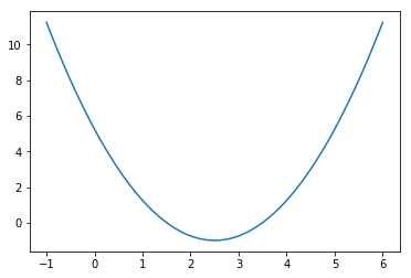

 

 

 

def dJ(theta):
    return 2*(theta-2.5)
​
def J(theta):
    try:
        return (theta-2.5)**2-1
    except:
        return float('inf')

　　

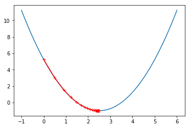
theta = 0.0
eta = 0.1
epsilon = 1e-8
​
while True:
    gradient =  dJ(theta)
    last_theta = theta
    theta = theta - eta * gradient
    if (abs(J(theta)-J(last_theta))<epsilon):
        break
print(theta)
print(J(theta))
>>>2.499891109642585
>>>-0.99999998814289

　　

theta = 0.0
eta = 0.1
epsilon = 1e-8
history = [theta]
​
while True:
    gradient =  dJ(theta)
    last_theta = theta
    theta = theta - eta * gradient
    history.append(theta)
    if (abs(J(theta)-J(last_theta))<epsilon):
        break
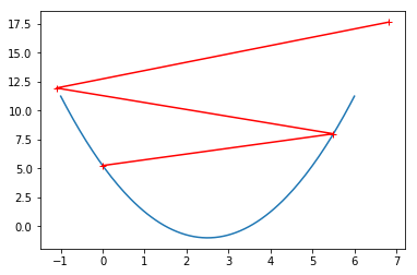
plt.plot(x,y)
plt.plot(np.array(history),J(np.array(history)),color='r',marker='+')
plt.show()
print("走的步数：%s"%(len(history)))

 

 

 

走的步数：46

 

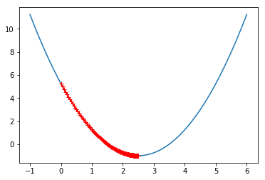
theta = 0.0
eta = 0.01
epsilon = 1e-8
history = [theta]
​
while True:
    gradient =  dJ(theta)
    last_theta = theta
    theta = theta - eta * gradient
    history.append(theta)
    if (abs(J(theta)-J(last_theta))<epsilon):
        break
plt.plot(x,y)
plt.plot(np.array(history),J(np.array(history)),color='r',marker='+')
plt.show()
print("走的步数：%s"%(len(history)))

　　

 

走的步数：424

 

theta = 0.0
eta = 0.8
epsilon = 1e-8
history = [theta]
​
while True:
    gradient =  dJ(theta)
    last_theta = theta
    theta = theta - eta * gradient
    history.append(theta)
    if (abs(J(theta)-J(last_theta))<epsilon):
        break
plt.plot(x,y)
plt.plot(np.array(history),J(np.array(history)),color='r',marker='+')
plt.show()
print("走的步数：%s"%(len(history)))

　　

 

走的步数：22

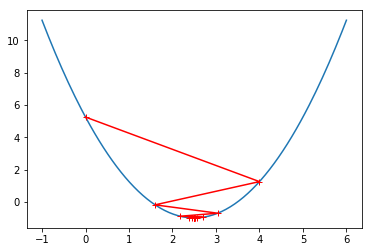
theta = 0.0
eta = 1.1
epsilon = 1e-8
history = [theta]
iters = 0
​
while True:
    iters += 1
    gradient =  dJ(theta)
    last_theta = theta
    theta = theta - eta * gradient
    history.append(theta)
    if (abs(J(theta)-J(last_theta))<epsilon or iters>=3):
        break
plt.plot(x,y)
plt.plot(np.array(history),J(np.array(history)),color='r',marker='+')
plt.show()
print("走的步数：%s"%(len(history)))

　

 

 

 

走的步数：4

 

在线性回归的模型中使用梯度下降

import numpy as np
import matplotlib.pyplot as plt
 

np.random.seed(5)
x = 2*np.random.random(size=100)
y = x*3+4+np.random.normal(size=100)
x = x.reshape((-1,1))
y.shape
 
 
>>>(100,)
 
plt.scatter(x,y)
plt.show()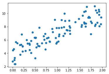

 

def J(theta,x,y):
    try:
        return np.sum(np.power((y - np.dot(x,theta)),2))/x.shape[0]
    except:
        return float('inf')
 
 
def dJ(theta,x,y):
    length = theta.shape[0]
    res = np.zeros(length)
    res[0] = np.sum(x.dot(theta)-y)
    for i in range(1,length):
        res[i] = np.sum((x.dot(theta)-y).dot(x[:,i]))
    return res*2/x.shape[0]
 

 
eta = 0.01
epsilon = 1e-8
iters = 0
x = np.hstack((np.ones((x.shape[0],1)),x))
theta = np.zeros([x.shape[1]])
x.shape
theta.shape
 
>>>(2,)
 
while True:
    iters += 1
    gradient =  dJ(theta,x,y)
    last_theta = theta
    theta = theta - eta * gradient
    if (abs(J(theta,x,y)-J(last_theta,x,y))<epsilon or iters>=10000):
        break
​
print(theta)
 
>>>[4.09099392 2.94805425]

　　

 

自己实现梯度下降多元线性回归:

class LinearRegressor:
    def __init__(self):
        self.coef_ = None # θ向量
        self.intercept_ = None # 截距
        self._theta = None
        self._epsilon = 1e-8
    def J(self,theta,x,y):
        try:
            return np.sum(np.power((y - np.dot(x,theta)),2))/len(x)
        except:
            return float('inf')
    def dJ(self,theta,x,y):
#         length = len(theta)
#         res = np.zeros(length)
#         res[0] = np.sum(x.dot(theta)-y)
#         for i in range(1,length):
#             res[i] = np.sum((x.dot(theta)-y).dot(x[:,i]))
#         return res*2/len(x)
        return x.T.dot(x.dot(theta)-y)*2/len(y)
​
    def fit(self,theta,x,y,eta):
        x = np.hstack((np.ones((x.shape[0],1)),x))
        iters = 0
        while True:
            iters += 1
            gradient =  self.dJ(theta,x,y)
            last_theta = theta
            theta = theta - eta * gradient
​
            if (abs(self.J(theta,x,y)-self.J(last_theta,x,y))<self._epsilon or iters>=10000):
                break
        self._theta = theta
        self.intercept_ = self._theta[0] # 截距
        self.coef_ = self._theta[1:] # 权重参数weights
        return self
    def predict(self,testX):
        x = np.hstack((np.ones((testX.shape[0],1)),testX))
#         y = np.dot(x,self._theta.reshape(-1,1))
        y = np.dot(x,self._theta)
        return y
    def score(self,testX,testY):
        return r2_score(testY,self.predict(testX))
 

 
lr = LinearRegressor()
theta = np.zeros([x.shape[1]+1])
lr.fit(theta,x,y,0.01)
print(lr.coef_)
print(lr.intercept_)
 
 
 
>>>[2.94805425]
>>>4.090993917959022

　　

 

随机梯度下降法:

 

1. 跳出局部最优解
2. 更快的运行速度

 

 

学习率随着循环次数而递减

import numpy as np
import matplotlib.pyplot as plt
 
 
m = 100000
​
x = np.random.normal(size=m)
X = np.reshape(x,(-1,1))
y = 4*x +3 +np.random.normal(0,3,size=m)
 
 

 
# 梯度下降法
 
lr = LinearRegressor()
theta = np.zeros([X.shape[1]+1])
%time lr.fit(theta,X,y,0.01)
print(lr.coef_)
print(lr.intercept_)
 
 
 
Wall time: 3.76 s
[3.99569098]
2.999661554158197
In [33]:
 
 
 
 
 
class StochasticGradientDescent(LinearRegressor):
    def dJ(self,theta,x_i,y_i):
        return x_i.T.dot(x_i.dot(theta)-y_i)*2
    def learn_rate(self,t):
        t0 = 5
        t1 = 50
        return t0/(t+t1)
    def fit(self,theta,x,y,eta,n=5):
​
        x = np.hstack((np.ones((x.shape[0],1)),x))
        iters = 0
        m = len(x)
       for i in range(n):  
            index = np.random.permutation(m)
            x_new = x[index]
            y_new = y[index]
            for j in range(m):
                rand_i = np.random.randint(len(x))
                gradient =  self.dJ(theta,x_new[rand_i],y_new[rand_i])
                theta = theta - self.learn_rate(eta) * gradient
​
        self._theta = theta
        self.intercept_ = self._theta[0] # 截距
        self.coef_ = self._theta[1:] # 权重参数weights
        return self
 
 
sgd = StochasticGradientDescent()
theta = np.zeros([X.shape[1]+1])
%time sgd.fit(theta,X,y,0.01)
print(sgd.coef_)
print(sgd.intercept_)
 
 
>>>Wall time: 3.86 s
>>>[4.21382386]
>>>2.2958068134016685
 
## scikit learn 的实现

 
from sklearn.linear_model import SGDRegressor
 

sgd = SGDRegressor(max_iter=5)
sgd.fit(X,y)
print(sgd.coef_)
print(sgd.intercept_)
 
 
 
>>>[3.99482988]
>>>[3.01943775]
 

　　

　　

梯度调试：

import numpy as np
import matplotlib.pyplot as plt
 
 
np.random.seed(seed=666)
x = np.random.random(size=(1000,10))
theta_true = np.arange(1,12,dtype=np.float32)
x_b = np.hstack([np.ones((x.shape[0],1)),x])
y = np.dot(x_b,theta_true) + np.random.normal(size=1000)
 
 
print(x.shape)
print(y.shape)
print(theta_true)
 
 
 
>>>(1000, 10)
>>>(1000,)
>>>[ 1.  2.  3.  4.  5.  6.  7.  8.  9. 10. 11.]

 
class Debug_GradientDescent(LinearRegressor):
    def dJ(self,theta,x,y):
        """导数的定义"""
        epsilon = 0.01
        res = np.empty(len(theta))
        for i in range(len(theta)):
            theta_1 = theta.copy()
            theta_1[i] += epsilon
            theta_2 = theta.copy()
            theta_2[i] -= epsilon
            res[i] = (self.J(theta_1,x,y) - self.J(theta_2,x,y))/(2*epsilon)
        return res
 
 
debug_gd = Debug_GradientDescent()
theta = np.zeros([x.shape[1]+1])
%time debug_gd.fit(theta,x,y,0.01)
debug_gd._theta
 
 
 
>>>Wall time: 14.5 s
>>>array([ 1.1251597 ,  2.05312521,  2.91522497,  4.11895968,  5.05002117,
        5.90494046,  6.97383745,  8.00088367,  8.86213468,  9.98608331,
       10.90529198])

 
lr = LinearRegressor()
theta = np.zeros([x.shape[1]+1])
%time lr.fit(theta,x,y,0.01)
lr._theta
 
 
 
>>>Wall time: 1.58 s

>>>array([ 1.1251597 ,  2.05312521,  2.91522497,  4.11895968,  5.05002117,
        5.90494046,  6.97383745,  8.00088367,  8.86213468,  9.98608331,
       10.90529198])

　　

 

 

 

 

 

​

 

 

 

转载于:https://www.cnblogs.com/zenan/p/9288658.html