实习中遇到的问题

●如何用http restful 发送请求request get 一个json数据?

import requests

response = requests.get('https://www.sojson.com/open/api/weather/json.shtml?city=北京',
                         )
print(response
      )

data = response.json()
print(data)

View Code

 

---

 

h2o的使用:

https://blog.csdn.net/gpwner/article/details/74058850

●如何运行?

这个代码需要安装jdk 8才行,安装9就不行.

# coding: utf-8

# In[1]:
#0411 84215599明天7点到10点空腹去体检
import h2o
h2o.init(port='2341')

View Code

然后浏览器中输入http://localhost:2341/就进入了

●之后按照上面博客的方法,就可以跑了.其中如何加入命令?点浏览器右边的outline点assist再点屏幕左边弹出来的importFiles就可以加入命令.或者直接点快捷栏最后一个圆圈问号图标也可以.

●h2o基本都鼠标操作就行了

决策树相关模型:

https://blog.csdn.net/google19890102/article/details/51746402/

●伯努利分布未必一定是 0-1 分布，也可能是 a-b 分布，只需满足相互独立、只取两个值的随机变量通常称为伯努利（Bernoulli）随机变量。二项分布就是n重伯努利分布

●随机森林效果不好,不如深度网络,最后用的gbm效果最好到百分之12

---

 

学习pytorch代码从github上.

clamp截断:

>>> a = torch.randn(4) >>> a  1.3869  0.3912 -0.8634 -0.5468 [torch.FloatTensor of size 4] >>> torch.clamp(a, min=-0.5, max=0.5)  0.5000  0.3912 -0.5000 -0.5000 [torch.FloatTensor of size 4]

---

●听同学大师说要通过github学习别人的代码.赶紧开始吧
●https://github.com/jcjohnson 很好的教程.
●项目1:做预测可以输出一个分布而不是一个数
●pytorch 和tensorflow 区别:
One aspect where static and dynamic graphs differ is control flow. For some models we may wi
sh to perform different computation for each data point; for example a recurrent network might be unrolled for different numbers of tim
e steps for each data point; this unrolling can be implemented as a loop. With a static graph the loop construct needs to be a part of th
e graph; for this reason TensorFlow provides operators such as
 tf.scan for embedding loops into the graph. With dynamic graphs the situation is simpler: since we build graphs on-the-fly for each exa
mple, we can use normal imperative flow control to perform computation that differs for each input.

 ●看看别人怎么做的预测问题:

1.把时间分成普通时间和特俗时间:比如双11,618,节假日等

搜集除已有销量数据之外的额外信息（比如天气、地点、节假日信息等），

https://blog.csdn.net/qq_19600291/article/details/74217896              很有启发

http://www.cnblogs.com/maybe2030/p/4585705.html

目前方法考虑:1.随即森林2.lstm

 

---

 

●https://blog.csdn.net/aliceyangxi1987/article/details/73420583  这个牛逼.

●这个keras写的真少,更好用.http://keras-cn.readthedocs.io/en/latest/

安装keras cuda版本:

conda install pip

pip install tensorflow-gpu

---

 

继续使用windows自带的linux.

0.安装好后,输入账号,密码.这时设置的是普通用户,比如zhangbo

1.第一次运行需要设置root账号

sudo passwd

之后设置好后就su root就可以切换root账号了.用这个账号就不用写sudo 了很方便但是比较危险.就是展示和配置文件时候用,其他时候不用.

2.普通使用的时候最好使用普通账号: su zhangbo 即可.

3.cmd改字体,标题上右键属性即可.

 #cpu keras库包的安装:https://blog.csdn.net/yangqiang200608/article/details/78719568?locationNum=9&fps=1

---

 

anaconda

Anaconda创建环境：

//下面是创建python=3.6版本的环境，取名叫py36

conda create -n py36 python=3.6 

 

删除环境（不要乱删啊啊啊）

conda remove -n py36 --all

 

激活环境

//下面这个py36是个环境名

source activate py36

 

退出环境

source deactivate

---

 

●2018-07-09  如何把代码封装成一个linux 的服务.使用的是windows的子系统ubuntu16版本.

1. 在/etc/init.d中vim myservice输入:

# -*- coding: utf-8 -*-
"""
Created on Mon Jul  9 19:37:31 2018

@author: 张博
"""
#!/bin/bash
#dcription: a demo
#chkconfig:2345 88 77
lockfile=/var/lock/subsys/myservice
touch $lockfile
# start
start(){
        if [ -e $lockfile ] ;then
                sh  ~/tmp.sh 
                echo "Service is already running....."
                return 5
        else
                touch $lockfile
                echo "Service start ..."
                return 0
        fi
}
#stop
stop(){
        if [ -e $lockfile ] ; then
                rm -f $lockfile
                echo "Service is stoped "
                return 0
        else
                echo "Service is not run "
                return 5
        fi
 
}
#restart
restart(){
        stop
        start
}
usage(){
        echo "Usage:{start|stop|restart|status}"
}
status(){
        if [ -e $lockfile ];then
                echo "Service is running .."
                return 0
        else
                echo "Service is stop "
                return 0
        fi
}
case $1 in
start)
        start
        ;;
stop)
        stop
        ;;
restart)
        restart
        ;;
status)
        status
        ;;
*)
        usage
        exit 7
        ;;
esac

View Code

2.在vim ~/tmp.sh输入:

echo 'dsfasdjlfs'

3. chmod+x /etc/init.d/myserver

4.service myservice start

5.屏幕输出:           也就是在服务里面运行了tmp.sh脚本,之所以把tmp.sh写在了~下,因为我测试过如果写在 /etc/init.d/中会提示无法打开tmp

dsfff
Service is already running..... 

以上实现了把代码封装到一个服务里面,这样只需要输入第四步代码就能运行程序tmp.sh

ps:对于windows的子系统.他们的文件系统共享的.c盘=/mnt/c       2个操作系统可以互相访问和修改文件  

---

 

  最后预测需要做的是

1.往服务器中装上需要的库包keras等

2..py封装成服务

 

---

●记录在linux系统中装keras环境.

 

4.

# 1. 更新系统包 sudo apt-get update sudo apt-get upgrade # 2. 安装Pip sudo apt-get install python-pip # 3. 检查 pip 是否安装成功 pip -V

pip install tensorflow

pip install keras

 

 

---

 

把上面服务的程序改成用python运行.

第一步改成

#!/bin/bash
#dcription: a demo
#chkconfig:2345 88 77
lockfile=/var/myservice.back
touch $lockfile
# start
start(){
        if [ -e $lockfile ] ;then
                python3  ~/tmp.py
                echo "Service is already running....."
                return 5
        else
                touch $lockfile
                echo "Service start ..."
                return 0
        fi
}
#stop
stop(){
        if [ -e $lockfile ] ; then
                rm -f $lockfile
                echo "Service is stoped "
                return 0
        else
                echo "Service is not run "
                return 5
        fi
 
}
#restart
restart(){
        stop
        start
}
usage(){
        echo "Usage:{start|stop|restart|status}"
}
status(){
        if [ -e $lockfile ];then
                echo "Service is running .."
                return 0
        else
                echo "Service is stop "
                return 0
        fi
}
case $1 in
start)
        start
        ;;
stop)
        stop
        ;;
restart)
        restart
        ;;
status)
        status
        ;;
*)
        usage
        exit 7
        ;;
esac

View Code

第二步改成:

在vim ~/tmp.py输入:

print('3232423')

---

 提示dpkg 被中断,您必须手工运行 sudo dpkg --configure -a解决此问题:

https://blog.csdn.net/ycl295644/article/details/44536297

---

 python 路径问题:

windows ,linux 都可以用

dataframe = read_csv(r'c:/nonghang/output998.csv',usecols=['Sum'])        这种写法来写路径,都不会报错

---

 

时间序列相关;

时间序列按变量分:绝对值时间序列,相对值时间序列,平均值时间序列

技巧:用差分来替换数据来去除趋势性,预测的干扰因素

# -*- coding: utf-8 -*-
"""
Created on Wed Jul 11 15:54:00 2018

@author: 张博
"""

#测试差分,确实可以消除趋势性,这样时间序列分析就更准确了.
a=[4,5,6,8,9,10,15,20]
b=[a[i+1]-a[i]   for i in range(len(a)) if i!=len(a)-1]
print(b)
import matplotlib.pyplot as plt
x=range(len(a))
plt.plot(x,a,c='red')
print(b)
x=range(len(b))
plt.plot(x,b)
plt.plot.show()

View Code

单调队列

 http://www.cnblogs.com/ECJTUACM-873284962/p/7301757.html#_labelTop

0,1背包变体:

#leecode461
class Solution:
    def canPartition(self, nums):
        """
        :type nums: List[int]
        :rtype: bool
        """
        if sum(nums)%2==1:
            return False
        tmp=sum(nums)//2
        memo={}
        def main(obj,list1):
              if (obj,tuple(list1)) in memo:
                    return memo[(obj,tuple(list1))]
              if obj!=0 and list1==[]:
                    return False
              if obj==0 :
                      return True
              if list1[0]>obj:
                return False
              for i in range(len(list1)):
                    if main(obj-list1[i],list1[:i]+list1[i+1:])==True:
                        memo[(obj,tuple(list1))]=True
                        return True
              memo[(obj,tuple(list1))]=False
              return False
        return main(tmp,nums)

View Code

 非常好的linux课程:

https://www.shiyanlou.com/courses/944

TCP\IP协议

https://www.shiyanlou.com/courses/98/labs/448/document

---

 

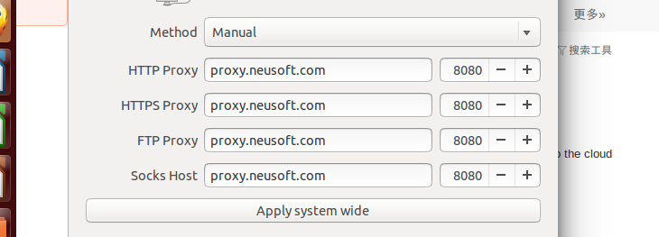
ubuntu 设置代理的方法:

vi /etc/apt/apt.conf

输入

Acquire::http::Proxy "http://账号:密码@代理地址:端口";

Acquire::http2::Proxy "http://账号:密码@代理地址:端口";

Acquire::ftp::Proxy "http://账号:密码@代理地址:端口";

 

 

 

之后就可以用apt-get 来通过代理下载软件了.ping 网站是ping不通的,因为这个方法只有apt有上网权限.

 好在:装keras linux 环境全用apt

这个方法在linux子系统里面可以使用.可能需要重新启动这个子系统让他生效.

 

sudo apt-get update  运行下这个必须

 

在虚拟机ubuntu14厘米也成功了.

 

改源

 https://blog.csdn.net/zgljl2012/article/details/79065174/

---

 安装显卡的tensorflow.

https://blog.csdn.net/weixin_39290638/article/details/80045236

我用的版本:cuda_9.0.176_win10        cudnn-9.1-windows10-x64-v7.1     (7.1版本的cudnn)

装好后会出现,找不到xxx.dll

这时候用管理员权限打开cmd.激活上面的tensorflow-gpu 这个conda环境.再测试就好使了.

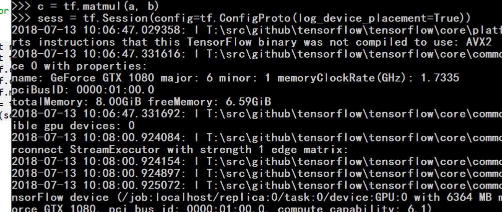
cmd里面运行session程序就能看到是不是用gpu了.

同时不用设置keras,他自动会使用gpu版本的tensorflow

●如何用编辑器来使用这个环境.进入anaconda navigator里面

从环境进入cmd.然后输入spyder即可.   ------------------------2018-07-13

 

---

 

python 追加写入: 用a+即可

 

with open('C:/Users/张博/Desktop/all.txt','a+') as f:

　　f.write('77777777777777777777777777777777777777')
　　f.write('\n')

 

---

● https://machinelearningmastery.com/time-series-forecasting-long-short-term-memory-network-python/

学习时间序列的处理方法:

1.要把数据stationary 化:用差分法

 2.高维的时间序列分析!效果最好的模型!:https://machinelearningmastery.com/multivariate-time-series-forecasting-lstms-keras/

    处理时间也是比1个变量慢非常多,但是效果很好,第一次跑农行数据没调参就低于百分之9的误差了.

---

 

●sublime多行编辑技巧:

1.ctrl+f 输入要查询的内容 再点find

2.alt+F3 全选查询内容

3.鼠标在文本框中点右键

4.鼠标在标题栏上点左键        这时就会出现很多个鼠标光标.就可以多光标输入了

---

 

●复习机器学习的算法:https://machinelearningmastery.com/start-here/#process

 

---

 

 

---

 

 

试试云Gpu主机:floydhub

发现上不去:网络不行.并且他给的配置也非常水

---

 

解决运行cnn网络出现:could not create cudnn handle: CUDNN_STATUS_NOT_INITIALIZED 的bug解决:

后来是下载的:cudnn-9.0-windows10-x64-v7.1   就可以了.把他解压缩到cuda 9.0文件夹里面覆盖即可.

这个包前面写9.0是cuda的标号,后面7.1是cudnn的标号.一定要对应好9.0的安装才行.

总结:tensorflow-gpu的安装.                   用的是cuda 9.0 版本, 和上面的cudnn就能跑了.配环境真是麻烦.

---

 

解决Proxifier和spyder冲突的问题:

用上proxifier 后发现python全不好使了.spder也不能用了.所以卸载proxifier 一切都好了.神奇一个代理软件居然能把python弄坏.

现在已经知道通过设置proxifier的代理规则即可,把一些软件设置为不用代理,比如spyder.这样就可以同时使用了.

 

---

 

●写bash脚本:

自己的ubuntu 16上面 

编写shell时，提示let：not found

解决方案: 用bash 1.sh 来运行脚本即可

 

---

 

把图片识别继续做下去:

1.多级文件夹的文件更名操作,为了名字不重复

from os import *
import os
#a='C:/Users/张博/Desktop/文件/图片项目'
#
#
#tmp=os.listdir(a)
#io=walk(tmp)
#print(io)
#dir_all=[]
#for i in tmp:
#    if path.isdir(a+'/'+i):
#        now_dir=a+'/'+i
#        dir_all.append(now_dir)
#print(dir_all) #得到第一层所有目录
#for i in range(1,11):
#  i=str(i)
#  b=a+'/after_process/'+i
#  if os.path.exists(b)==False:
#   os.makedirs(a+'/after_process/'+i)#递归的创建目录
import shutil

#shutil.copyfile("1.txt","3.txt")
   




shutil.copyfile("1.txt","3.txt")

path1='E:/pic2'
tmp=os.listdir(path1)
print(tmp)
tmp=[path1+'/'+i for i in tmp ]
print(os.path.isdir('E:/pic2'))
tmp=[i for i in tmp if path.isdir(i)]
print(tmp)
print(len(tmp))
a8=1
for i in tmp:
    jj=i
    now=listdir(jj)
    now=[ii for ii in now if path.isdir(i+'/'+ii)]
    now=[i+'/'+ii for ii in now ]
    print(now)
    
#    os.rename()
    for iii in now:
        a=os.path.abspath(iii)
        print(a)
        print(listdir(a))
        for i in listdir(a):
            print(a)
            print(type(a))
            out=a
            out=out+'\\'+i  #注意要写\\ 转义
            os.rename(out,out[:-4]+str(a8)+'.png')
            a8+=1
            
#终于何斌了.曹饿了7千多个图片
            
            
        





#for i in dir_all:
#    for j in os.listdir(i):
#        tmp=i+'/'+j
#        if path.isdir(tmp):
#            #i是P1,j是G1   i是包的标记,j是分类
#            k=os.listdir(tmp)
##           k= ['R10_l.png', 'R10_r.png', 'R11_l.png', 'R11_r.png', 'R12_l.png', 'R12_r.png', 'R13_l.png', 'R13_r.png', 'R14_l.png', 'R14_r.png', 'R15_l.png', 'R15_r.png', 'R16_l.png', 'R16_r.png', 'R17_l.png', 'R17_r.png', 'R18_l.png', 'R18_r.png', 'R19_l.png', 'R19_r.png', 'R1_l.png', 'R1_r.png', 'R20_l.png', 'R20_r.png', 'R2_l.png', 'R2_r.png', 'R3_l.png', 'R3_r.png', 'R4_l.png', 'R4_r.png', 'R5_l.png', 'R5_r.png', 'R6_l.png', 'R6_r.png', 'R7_l.png', 'R7_r.png', 'R8_l.png', 'R8_r.png', 'R9_l.png', 'R9_r.png']
#            print(k)
##            for kk in k:
##                
##                os.system("ren kk kk[:-4]+i[-2:]+'.png'")
##                print(kk)
##                fffffffffffffffffff
##            os.system()
#          










        
        
        
        

View Code

 2.拆分数据为test和valid

# -*- coding: utf-8 -*-
"""
Created on Sun Jul 15 17:48:36 2018

@author: 张博
"""

'''
右键属性,我们发现每一个图报里面有760张图片.足够了.如果不够还可以继续用keras的
图片生成器来随机对图片进行平移和旋转放缩操作来对图像进行提升.提升术语说的意思是
把一个图片通过这3个变换来生成很多相类似的图片,把这些图片也作为数据集,这样训练效果会跟好
更入帮性.
'''
from os import *
import shutil
a='C:/Users/张博/Desktop/图片总结/all_pic'
aa=listdir(a)
print(a)
a=[a+'/'+i for i in aa]
print(a)
for i in a:
    #i 是当前文件夹
    print(i)
    tmp=listdir(i)
    num=(760*2//3)
    test=tmp[:num]
    valid=tmp[num:]
    mkdir(i+'/'+'test')
    mkdir(i+'/'+'valid')
    for ii in test:
     shutil.move(i+'/'+ii,i+'/'+'test')          #移动文件
    for ii in valid:
     shutil.move(i+'/'+ii,i+'/'+'valid')          #移动文件
    
    
    
    
    
    
    
    
    
    
    
    
    

View Code

3.跑到93正确率:当然还有正则化,bn层还没加入.

from keras.preprocessing.image import ImageDataGenerator, array_to_img, img_to_array, load_img








##图像预处理:
#datagen = ImageDataGenerator(
#        rotation_range=10,
#        width_shift_range=1,
#        height_shift_range=1,
#        shear_range=0,
#        zoom_range=0.1,
#        horizontal_flip=True,
#        fill_mode='nearest')
# 
#img = load_img(r'C:/Users/张博/Desktop/cat.png')  # this is a PIL image
#x = img_to_array(img)  # this is a Numpy array with shape (3, 150, 150)
#
#print(x.shape)
##下面的方法把3维图片变4维图片
#x = x.reshape((1,) + x.shape)  # this is a Numpy array with shape (1, 3, 150, 150)#这个方法直接加一维
#
#print(x.shape)
## the .flow() command below generates batches of randomly transformed images
## and saves the results to the `preview/` directory
#i = 0
#for batch in datagen.flow(x, batch_size=1,
#                          save_to_dir='C:/Users/张博/Desktop/cat', save_prefix='cat'#默认的生成文件名前缀
#                          , save_format='png'):
#    i += 1
#    if i > 2:
#        break  # otherwise the generator would loop indefinitely
        
#img=load_img(r'C:/Users/张博/Desktop/cat/cat777777_0_1154.png')
#x = x.reshape((1,) + x.shape)
#print(x.shape)



from keras import backend as K
K.set_image_dim_ordering('th')
'''
if "image_dim_ordering": is "th" and "backend": "theano", your input_shape must be (channels, height, width)
if "image_dim_ordering": is "tf" and "backend": "tensorflow", your input_shape must be (height, width, channels)
因此上面我们需要设置 把模式切换成为'th'  .这点要注意.
'''











      
#搭建网络:

from keras.models import Sequential
from keras.layers import Convolution2D, MaxPooling2D
from keras.layers import Activation, Dropout, Flatten, Dense
 
model = Sequential()
model.add(Convolution2D(32, 3, 3, input_shape=(3, 150, 150)))
model.add(Activation('relu'))
model.add(MaxPooling2D(pool_size=(2, 2)))
 
model.add(Convolution2D(32, 3, 3))
model.add(Activation('relu'))
model.add(MaxPooling2D(pool_size=(2, 2)))
 
model.add(Convolution2D(64, 3, 3))
model.add(Activation('relu'))

model.add(MaxPooling2D(pool_size=(2, 2)))
 
# the model so far outputs 3D feature maps (height, width, features)





model.add(Flatten())  # this converts our 3D feature maps to 1D feature vectors
model.add(Dense(64))
model.add(Activation('relu'))
model.add(Dropout(0.5))
model.add(Dense(10)) #因为我们分10累所以最后这里写10

model.add(Activation("softmax")) #softmax可以把10这个向量的分类凸显出来
 



'''
我现在所知道的解决方法大致只有两种，第一种就是添加dropout层，dropout的原理我就不多说了，
主要说一些它的用法，dropout可以放在很多类层的后面，用来抑制过拟合现象，常见的可以直接放在Dense层后面，
对于在Convolutional和Maxpooling层中dropout应该放置在Convolutional和Maxpooling之间，还是Maxpooling
后面的说法，我的建议是试！这两种放置方法我都见过，但是孰优孰劣我也不好说，但是大部分见到的都是放在
Convolutional和Maxpooling之间。关于Dropout参数的选择，这也是只能不断去试，但是我发现一个问题，
在Dropout设置0.5以上时，会有验证集精度普遍高于训练集精度的现象发生，但是对验证集精度并没有太大影响，
相反结果却不错，我的解释是Dropout相当于Ensemble，dropout过大相当于多个模型的结合，一些差模型会拉低
训练集的精度。当然，这也只是我的猜测，大家有好的解释，不妨留言讨论一下。 
当然还有第二种就是使用参数正则化，也就是在一些层的声明中加入L1或L2正则化系数，




keras.layers.normalization.BatchNormalization(
epsilon=1e-06, mode=0, axis=-1, momentum=0.9, weights=None, beta_init='zero',
 gamma_init='one')

'''






# this is the augmentation configuration we will use for training
train_datagen = ImageDataGenerator(
        rescale=1./255,
        shear_range=0.2,
        zoom_range=0.2,
        horizontal_flip=True)
 
# this is the augmentation configuration we will use for testing:
# only rescaling
test_datagen = ImageDataGenerator(rescale=1./255)
 
# this is a generator that will read pictures found in
# subfolers of 'data/train', and indefinitely generate
# batches of augmented image data



train_generator = train_datagen.flow_from_directory(
        'C:/Users/张博/Desktop/图片总结/all_pic/test',  # this is the target directory
        target_size=(150, 150),  # all images will be resized to 150x150
        batch_size=20,          #说一般不操过128,取16,32差不多
        class_mode='sparse')  # since we use binary_crossentropy loss, we need binary labels




# this is a similar generator, for validation data
validation_generator = test_datagen.flow_from_directory(
        'C:/Users/张博/Desktop/图片总结/all_pic/valid',
        target_size=(150, 150),
        batch_size=20,
        class_mode='sparse')


#learning rate schedual 太重要了.经常发现到最后的学习效果提升很慢了.就是因为步子太大了扯蛋了.
def schedule(epoch):
    rate=0.7
    if epoch<3:
        return 0.002  #开始学的快一点
    if epoch<10:
        return 0.001
    if epoch<20:
        return 0.001*rate
    if epoch<30:
        return 0.001*rate**2
    if epoch<100:
       return 0.001*rate**3
    else:
        return 0.001*rate**4
    
learning_rate=keras.callbacks.LearningRateScheduler(schedule)
learning_rate2=keras.callbacks.ReduceLROnPlateau(factor=0.7)


adam=keras.optimizers.Adam( beta_1=0.9, beta_2=0.999, epsilon=1e-08,clipvalue=0.5)#lr=0.001
model.compile(loss='sparse_categorical_crossentropy',
              optimizer=adam,
              metrics=['accuracy'])



#https://www.cnblogs.com/bamtercelboo/p/7469005.html       非常nice的调参总结


H=model.fit_generator(
        train_generator,
        steps_per_epoch=2000,     #  一个epoch训练多少次生成器给的数据,无所谓随便写一个就行,
                                  #也就是说一个epoch要训练多久,无所谓的一个数,但是如果看效果着急就设小一点.
        nb_epoch=500,         #总工迭代多少轮,越大越好
        validation_data=validation_generator,callbacks=[learning_rate,
         learning_rate2]
        )
 
#其实对于这个10分类问题就看acc指数就够了

print(H.history["loss"])
print(H.history["val_loss"])
print(H.history["acc"])


'''
batch的理解:
    有一堆人各种需求,总体放进去算loss函数肯定能让所有人的满意度提升
    但是人太多了,超大规模矩阵算梯度太慢了,所以选一小组人batch作为训练就可以了,让他们满足就行了.
    因为数据经过shuffle,所以每一次取得小组基本能代表所有人的需求.所以batch取大一点更能反映整体性质.
    但是单步计算可能就慢一些.所以一般16到100之见做选择.
'''




















        
        
        
        

View Code

等训练好了,写一个调参总结,把参数大概取什么范围定下来.其中动态学习率非常重要.

  

---

 

 

mysql傻瓜式安装:

https://blog.csdn.net/NepalTrip/article/details/79492058

我选择的版本是:

安装步奏:狂next,运行:不过每次使用的时候，必须进入mysql的安装bin目录才可以通过mysql -u root -p 进入.成功进入.

如果发现进不去就是因为mysql的服务没有开启,开启即可.

不好使可以试试:C:\Program Files\MySQL\MySQL Server 5.7\bin\mysql.exe 这个直接进

 

 

---

 复习到逻辑回归的对数loss函数不是很理解.去找书看看怎么推导的.

发现周志华的书上推导错了,极大思然写的不对,推导其实就是极大思然的公式带进去就完了. 一个2项分布的释然函数而已

似然函数=p1^(y1)*(1-p1)^y0 就对了.

---

 记录solr的使用方法:

1.http://localhost:8080/solr/index.html#/           进入solr界面

2.接下来就是创建solrCore

   在solrHome,我们创建一个空文件夹core1，

    把solrHome里面有别人的账号,把他的conf文件夹贴到core1里面.

    在solr的管理控制台界面 --core Admin   ----Add Core

3.需要做的东西是把csv文件都放到solr服务器上.因为solr只能存.json 所以这里用了pysolr这个库包.

下面实现了这个上传csv到solr的功能.ps:这个库包还可以维护solr

'''
文档:https://pypi.org/project/pysolr/3.3.0/
localhost后面没有.com
'''
from __future__ import print_function
import csv
import csv,json
b=csv.reader(open(r'C:\Users\张博\Desktop\solr_test.csv'))

b=list(b)
c=b[0]
keys=c

out=[]
for i in range(1,len(b)):
    tmp=b[i]
    out.append(dict(zip(keys,tmp)))

##a=json.dumps( out ,indent=4)
##print(a)
##
##










import pysolr
#这个url很重要，不能填错了
##solr = pysolr.Solr('http://localhost:8080/solr/jcg/', timeout=10)
solr = pysolr.Solr('http://localhost:8080/solr/index.html#/zhangbo/documents', timeout=10)


'''
插入:
'''

#正确的数据格式，可以少项
##solr.add([
##    {
##        "id": "doc_1",
##        "name": "A test document",
##        "cat": "book",
##        "price": "7.99",
##        "inStock": "T",
##        "author": "George R.R. Martin",
##        "series_t": "A Song of Ice and Fire",
##        "sequence_i": "1",
##        "genre_s": "fantasy",
##    }
##])




'''
取数据


'''


# Setup a basic Solr instance. The timeout is optional.
solr = pysolr.Solr('http://localhost:8080/solr/zhangbo', timeout=10)

solr.delete(q='*:*')
results = solr.search('*:*')
print(list(results.__dict__))
print('打印完了')
# How you would index data.
solr.add(out)
print('added')


#搜索jcg中的全部数据
results = solr.search('*:*')

###搜索id为doc_1的数据
##doc1 = solr.search('id:doc_1')


print(results.__dict__)




'''
#删除id为doc_1的数据
solr.delete(id='doc_1') 

#删除所有数据
solr.delete(q='*:*')
'''

View Code

 下面实现,用pysolr对solr进行控制,包括高级搜索功能!

#从solr中读取jason格式的数据



import pysolr
#这个url很重要，不能填错了
##solr = pysolr.Solr('http://localhost:8080/solr/jcg/', timeout=10)
solr = pysolr.Solr('http://localhost:8080/solr/index.html#/zhangbo/documents', timeout=10)
print(423)

'''
插入:
'''

#正确的数据格式，可以少项
##solr.add([
##    {
##        "id": "doc_1",
##        "name": "A test document",
##        "cat": "book",
##        "price": "7.99",
##        "inStock": "T",
##        "author": "George R.R. Martin",
##        "series_t": "A Song of Ice and Fire",
##        "sequence_i": "1",
##        "genre_s": "fantasy",
##    }
##])





'''
取数据


'''
solr = pysolr.Solr('http://localhost:8080/solr/zhangbo', timeout=10)

#一定要在这个地址的solr上操作.
solr.delete(q='*:*')
print(324234)
solr.add([
    {
        "idd": "doc_1",
        "title": "A",
        
    },
    {
        "idd": "doc_2",
        "title": "B",
        
    },
    {
        "idd": "doc_1",
        "title": "C",
        
    },
])


#打印全部
print(list(solr.search('*:*')))

'''

#测试了一天,可算试出来如何高级搜索了.遇到问题可以看这个py库的源码.

#这个search函数的原理是**kwarg传入一个字典.字典的key是查询的命令,

#value是你要查询命令的输入框中应该写入的内容.也是从csdn

https://blog.csdn.net/sinat_33455447/article/details/63341339

这个网页受到的启示.他写的是start后面接页数,所以对应改fq,后面就是接一个条件.



'''     

doc1 = solr.search("idd:doc_1" , **{"fq":'title:A'})



#读取之后需要list一下,会自动去掉垃圾信息
doc1=list(doc1)

print(doc1)




# Setup a basic Solr instance. The timeout is optional.



print('打印完了')

View Code

 4.批量传输最后用的这个脚本:

'''
文档:https://pypi.org/project/pysolr/3.3.0/
localhost后面没有.com
'''
from __future__ import print_function
import csv
import csv,json
b=csv.reader(open(r'C:\Users\张博\Desktop\201707\20170701.csv'))

b=list(b)
c=b[0]
keys=c
import pysolr
out=[]
print('kaishi' )
solr = pysolr.Solr('http://localhost:8080/solr/zhangbo', timeout=10)

#先都删了
solr.delete(q='*:*')



j=1
while j <len(b) :
    print('当前放入第%s个到%s+1000)个'%(j,j))
    tmp2=b[j:j+1000]
    for i in tmp2:
        tmp=i
        out.append(dict(zip(keys,tmp)))
        
        
        # How you would index data.
    solr.add(out)    
        
        


        
    j+=1000
    out=[]

import pysolr
# Setup a basic Solr instance. The timeout is optional.



##a=json.dumps( out ,indent=4)
##print(a)
##
##










import pysolr
#这个url很重要，不能填错了
##solr = pysolr.Solr('http://localhost:8080/solr/jcg/', timeout=10)


'''
插入:
'''

#正确的数据格式，可以少项
##solr.add([
##    {
##        "id": "doc_1",
##        "name": "A test document",
##        "cat": "book",
##        "price": "7.99",
##        "inStock": "T",
##        "author": "George R.R. Martin",
##        "series_t": "A Song of Ice and Fire",
##        "sequence_i": "1",
##        "genre_s": "fantasy",
##    }
##])




'''
取数据


'''




###搜索jcg中的全部数据
##results = solr.search('*:*')
##
#####搜索id为doc_1的数据
####doc1 = solr.search('id:doc_1')
##
##
##
##
##
##
##
##'''
###删除id为doc_1的数据
##solr.delete(id='doc_1') 
##
###删除所有数据
##solr.delete(q='*:*')
##'''
##
##
##
##
##
##
##
##

View Code

 

---

 

2018-07-17,10点52  lstm继续做下去

1.处理数据,加入特征

# -*- coding: utf-8 -*-
"""
Created on Tue Jul 17 10:48:30 2018

@author: 张博
"""

# -*- coding: utf-8 -*-
"""
Created on Tue Jul 17 09:26:35 2018

@author: 张博
"""



import pandas as pd

#把所有数据拼起来从1到30,这次先不把星期6,日排除
print(3423)
list_all=[]
for i in range(1,31):
     if i<10:
         index_now=str(0)+str(i)
     else:
         index_now=str(i)
     path='C:/Users/张博/Desktop/201707/201707'+index_now+'.csv'
     #路径带中文会报错,改用下面的方法
     f = open(path)
     tmp=pd.read_csv(f)
     f.close()
     list_all.append(tmp)
all_data=pd.concat(list_all)


print(34234)

#选取部分数据,注意'ret_code'里面有空格

#把省份拆开,对不同省份做不同的预测.最后需要预测哪个省份就把哪个省份的数据扔给那个省份的训练器
data=all_data #现在data是全部30天的数据了,经过测试还是用两个条件一起对data做拆分更好.比只用Province好.
a=data['Province']==99 
b=data['ret_code']=='N         '

c=a&b
tmp=data[c]
#tmp 就是99,N这个条件下的数据汇总

#下面把小时合并起来
#首先得到所有可能结果的分类然后query即可

print('over')

print(set(tmp['YY']))
list=[]
for yy in set(tmp['YY']):
    for mm in set(tmp['MM']):
        for dd in set(tmp['DD']):
            for hh in set(tmp['HH']):
                now=tmp.query('YY==@yy and MM==@mm and DD==@dd and HH==@hh')
                a=now['sum(BPC_BOEING_201707_MIN.cnt)'].sum()
                #创建一个表
                #下面就是创建一个表的写法
                df = pd.DataFrame([{'YY':yy, 'MM':mm,'DD':dd,'HH':hh,'Province':99,'ret_code':'N', 'Sum':a}]
                                  ,columns =['YY','MM','DD','HH','Province','ret_code','Sum'])
                
                list.append(df)
a=pd.concat(list)
#a.to_csv(r'e:\output_nonghang\output998.csv')
#到这里得到了700多行数据,下面利用这700多行数据预测31号24小时的99_N的交易量


'''
奇怪存一下读一下才好用.非常神秘!!!!
'''
print(type(a))                
a.to_csv(r'e:\output_nonghang\output998.csv')
print(type(a))
a=pd.read_csv(r'e:\output_nonghang\output998.csv')




import pandas as pd




a['holiday']=0
#a=a.loc(a['DD'].isin([1,2,8,9,15,16,22,23,29,30]))
#help(a)
#print(a)
#遍历


for i in range(len(a)):
    if a.loc[i,'DD'] in [1,2,8,9,15,16,22,23,29,30]:
        a.loc[i,'holiday']=1

a.to_csv(r'e:\output_nonghang\out.csv')
a=a[['DD','HH','holiday','Sum']]
print(len(a))
print(len(a.loc[0]))
print(a)
a.to_csv(r'e:\output_nonghang\out.csv',index=None)

#下面利用这个数据,总共4个特征来对最后一个特征sum来做预测.

'''
跑完这个程序我们得到饿了out.csv
这个数据表示99,N这个类型的数据他的4个特征组成的数据
'''

View Code

 

 

 

---

 

sublime编辑技巧:

按住shift,鼠标右键拉框.就能多行编辑,想选哪里就选哪里 

 

 

 

 

---

 

2018-07-17,20点10 对lstm预测项目的总结:

通过学习积累了处理大数据基本方法

1.要把原始数据的图像画出来,做大体走势和噪音点的分析.

 

从图片中我们看出其中23号的数据非常低,查看数据发现他凌晨3点数据是3千,比浅一天3点数据小了80被.而恰巧按照时间序列的原则去掉最前面的一部分数据(因为他没有历史值),用其他数据的后三分之一做预测,正好包含了这个点的数据.所以导致最后预测的效果不好.

2.对于时间序列的预测可以采用多元lstm.

参考:https://machinelearningmastery.com/multivariate-time-series-forecasting-lstms-keras/

# -*- coding: utf-8 -*-
"""
Created on Tue Jul 17 10:54:38 2018

@author: 张博
"""

# -*- coding: utf-8 -*-
"""
Created on Mon Jul 16 17:18:57 2018

@author: 张博
"""

# -*- coding: utf-8 -*-
"""
Spyder Editor

This is a temporary script file.
"""











#老外的教程:非常详细,最后的多变量,多step模型应该是最终实际应用最好的模型了.也就是这个.py文件写的内容
#https://machinelearningmastery.com/multivariate-time-series-forecasting-lstms-keras/

'''
SUPER_PARAMETER:一般代码习惯把超参数写最开始位置,方便修改和查找
'''
EPOCH=1
LOOK_BACK=24
n_features = 4         #这个问题里面这个参数不用动,因为只有2个变量

n_hours = LOOK_BACK


import pandas as pd

from pandas import read_csv
from datetime import datetime
# load data
def parse(x):
    return datetime.strptime(x, '%Y %m %d %H')
data = read_csv(r'E:\output_nonghang\out.csv')


#切片和concat即可
tmp1=data.iloc[:,:3]
tmp2=data.iloc[:,3]

print(tmp1)
print(tmp2)
print(type(tmp1))
data=pd.concat([tmp2,tmp1],axis=1)
print(data)


#因为下面的模板是把预测值放在了第一列.所以对data先做一个变换.













#data.to_csv('pollution.csv')






from pandas import read_csv
from matplotlib import pyplot
# load dataset
dataset = data
values = dataset.values



# specify columns to plot
groups = [0, 1, 2, 3, 5, 6, 7]
i = 1


from pandas import read_csv
from matplotlib import pyplot
# load dataset
#dataset = read_csv('pollution.csv', header=0, index_col=0)
##print(dataset.head())
#values = dataset.values
# specify columns to plot
#groups = [0, 1, 2, 3, 5, 6, 7]
#i = 1
# plot each column
#pyplot.figure()
#图中每一行是一个列数据的展现.所以一共有7个小图,对应7个列指标的变化.
#for group in groups:
#    pyplot.subplot(len(groups), 1, i)
#    pyplot.plot(values[:, group])
#    pyplot.title(dataset.columns[group], y=0.5, loc='right')
#    i += 1
##pyplot.show()



from math import sqrt
from numpy import concatenate
from matplotlib import pyplot
from pandas import read_csv
from pandas import DataFrame
from pandas import concat
from sklearn.preprocessing import MinMaxScaler
from sklearn.preprocessing import LabelEncoder
from sklearn.metrics import mean_squared_error
from keras.models import Sequential
from keras.layers import Dense
from keras.layers import LSTM
# load dataset
dataset = read_csv('pollution.csv', header=0, index_col=0)
values = dataset.values
# integer encode direction
#把标签标准化而已.比如把1,23,5,7,7标准化之后就变成了0,1,2,3,3
#print('values')
#print(values[:5])
#encoder = LabelEncoder()
#values[:,4] = encoder.fit_transform(values[:,4])
## ensure all data is float
#values = values.astype('float32')
#print('values_after_endoding')
#numpy 转pd
import pandas as pd
#pd.DataFrame(values).to_csv('values_after_endoding.csv')
#从结果可以看出来encoder函数把这种catogorical的数据转化成了数值类型,
#方便做回归.
#print(values[:5])
# normalize features,先正规化.
scaler = MinMaxScaler(feature_range=(0, 1))
scaled = scaler.fit_transform(values)
print('正规化之后的数据')

pd.DataFrame(scaled).to_csv('values_after_normalization.csv')

# frame as supervised learning




# convert series to supervised learning
#n_in:之前的时间点读入多少,n_out:之后的时间点读入多少.
#对于多变量,都是同时读入多少.为了方便,统一按嘴大的来.
#print('测试shift函数')
#
#df = DataFrame(scaled)
#print(df)      # 从测试看出来shift就是数据同时向下平移,或者向上平移.
#print(df.shift(2))
def series_to_supervised(data, n_in=1, n_out=1, dropnan=True):
    n_vars = 1 if type(data) is list else data.shape[1]
    df = DataFrame(data)
    cols, names = [],[]
    # input sequence (t-n, ... t-1)
    for i in range(n_in, 0, -1):
        cols.append(df.shift(i))
        names += [('var%d(时间:t-%s)' % (j+1, i)) for j in range(n_vars)]
    # forecast sequence (t, t+1, ... t+n)
    for i in range(0, n_out):
        cols.append(df.shift(-i))
        if i == 0:
            names += [('var%d(时间:t)' % (j+1)) for j in range(n_vars)]
        else:
            names += [('var%d(时间:t+%d)' % (j+1, i)) for j in range(n_vars)]
    # put it all together
    agg = concat(cols, axis=1)
    agg.columns = names
    # drop rows with NaN values
    if dropnan:
        agg.dropna(inplace=True)
    return agg




















#series_to_supervised函数把多变量时间序列的列拍好.

reframed = series_to_supervised(scaled, LOOK_BACK, 1)
print(reframed.shape)
# drop columns we don't want to predict
#我们只需要预测var1(t)所以把后面的拍都扔了.








# split into train and test sets
values = reframed.values
n_train_hours = int(len(scaled)*0.67)
train = values[:n_train_hours, :]
test = values[n_train_hours:, :]
# split into input and outputs
n_obs = n_hours * n_features
train_X, train_y = train[:, :n_obs], train[:, -n_features]
test_X, test_y = test[:, :n_obs], test[:, -n_features]
#print(train_X.shape, len(train_X), train_y.shape)
#print(test_X.shape, len(test_X), test_y.shape)
#print(train_X)
#print(9999999999999999)
#print(test_X)












#这里依然是用timesteps=1
#从这个reshape可以看出来,之前的单变量的feature长度=look_back
#                       现在的多变量feature长度=look_back*len(variables).就这一个区别.
# reshape input to be 3D [samples, timesteps, features]
train_X = train_X.reshape((train_X.shape[0], n_hours, n_features))
test_X = test_X.reshape((test_X.shape[0], n_hours, n_features))
#print(train_X.shape, train_y.shape, test_X.shape, test_y.shape)

'''
网络结构比较小的时候，效率瓶颈在CPU与GPU数据传输，这个时候只用cpu会更快。
网络结构比较庞大的时候，gpu的提速就比较明显了。


:显存和内存一样,属于随机存储,关机后自动清空。
'''



print('开始训练')

# design network
model = Sequential()
import keras
from keras import regularizers

from keras import optimizers

import keras

model.add(keras.layers.recurrent.GRU(77, input_shape=(train_X.shape[1], train_X.shape[2]),activation='tanh', 
                                     recurrent_activation='hard_sigmoid',
                                     kernel_regularizer=regularizers.l2(0.01),
                                     recurrent_regularizer=regularizers.l2(0.01)
                                     , bias_regularizer=regularizers.l2(0.01), 
                                     dropout=0.2, recurrent_dropout=0.2))

#model.add(Dense(60, activation='tanh',kernel_regularizer=regularizers.l2(0.01),
#                bias_regularizer=regularizers.l2(0.01)))



def schedule(epoch):
    rate=0.3
    if epoch<3:
        return 0.002  #开始学的快一点
    if epoch<10:
        return 0.001
    if epoch<20:
        return 0.001*rate
    if epoch<30:
        return 0.001*rate**2
    if epoch<70:
       return 0.001*rate**3
    else:
        return 0.001*rate**4
import keras
learning_rate=keras.callbacks.LearningRateScheduler(schedule)
learning_rate2=keras.callbacks.ReduceLROnPlateau(factor=0.5)
#input_dim：输入维度，当使用该层为模型首层时，应指定该值（或等价的指定input_shape)

model.add(Dense(1, activation='tanh'))

#loss:mse,mae,mape,msle
adam = optimizers.Adam(lr=0.001, clipnorm=1.)
model.compile(loss='mape', optimizer=adam)
# fit network
#参数里面写validation_data就不用自己手动predict了,可以直接画histrory图像了
history = model.fit(train_X, train_y, epochs=EPOCH, batch_size=1,
                    validation_data=(test_X, test_y),
                    verbose=2, shuffle=False,callbacks=[learning_rate,
         learning_rate2])
# plot history
pyplot.plot(history.history['loss'], label='train')
pyplot.plot(history.history['val_loss'], label='test')
pyplot.legend()
pyplot.show()



#训练好后直接做预测即可.
# make a prediction
yhat = model.predict(test_X)         #yhat 这个变量表示y上面加一票的数学符号
                             #在统计学里面用来表示算法作用到test上得到的预测值
test_X = test_X.reshape((test_X.shape[0], n_hours*n_features))
# invert scaling for forecast







#因为之前的scale是对初始数据做scale的,inverse回去还需要把矩阵的型拼回去.
inv_yhat = concatenate((yhat, test_X[:, -(n_features-1):]), axis=1)
inv_yhat = scaler.inverse_transform(inv_yhat)
inv_yhat = inv_yhat[:,0]#inverse完再把数据扣出来.多变量这个地方需要的操作要多点
# invert scaling for actual



print(test_y)
print(99999999999)
test_y = test_y.reshape((len(test_y), 1))
inv_y = concatenate((test_y, test_X[:, -(n_features-1):]), axis=1)
inv_y = scaler.inverse_transform(inv_y)
inv_y = inv_y[:,0]














# calculate RMSE
rmse = sqrt(mean_squared_error(inv_y, inv_yhat))

print('输出abs差百分比指标:')
#这个污染指数还有0的.干扰非常大
#print(inv_y.shape)
#print(inv_yhat.shape)
wucha=abs(inv_y-inv_yhat)/(inv_y+0.1)
#print(wucha)


#with open(r'c:/234/wucha.txt','w') as f:
#      print(type(wucha))
#      wucha2=list(wucha)
#      wucha2=str(wucha2)
#      f.write(wucha2)




wucha=wucha.mean()
print(wucha)



inv_y=inv_y
inv_yhat=inv_yhat

#print('Test RMSE: %.3f' % rmse)
import numpy as np


pyplot.plot(inv_y,color='black')
pyplot.plot(inv_yhat     ,color='red')

pyplot.show()




'''
写文件的模板
with open(r'c:/234/wucha.txt','w') as f:
      wucha=str(wucha)
      f.write(wucha)
'''



'''
下面对于lookback参数应该设置多少进行测试:
因为有些数据是0对abs百分比影响很大.所以还是用rms来做指标:
lookback=1:    rmse:26.591
lookback=30      Test RMSE: 26.124
'''


'''
手动加断电的方法:raise NameError #这种加断点方法靠谱
'''

'''
画图模板:
from matplotlib import pyplot
data=[]
pyplot.plot(inv_y,color='black')


pyplot.show()

'''

View Code

 3.最后误差百分之8.4  mape

 

3.调参和模型:

数据初始要正则化,动态学习率,参数的初始化和正则化,通过history方法可以观察是否过拟合.提高gpu使用率:可以用不同ide同时跑python程序.

其实都用cmd来跑也可以.cmd可以同时运行多个python互相不干扰.这样gpu利用率高多了.能提高调参效率

 

---

 

https://machinelearningmastery.com/cnn-long-short-term-memory-networks/

这个应该试试.

 

---

 

windows 里面安装\卸载 子系统ubuntu.出错了就卸载重装

https://blog.csdn.net/shixuehancheng/article/details/52173267

 

---

 

https://www.cnblogs.com/shellway/p/3699982.html                    java例子

 

---

 

记录java:

Syntax error on token "Invalid Character", delete this token     Syntax error on tokens, delete these tokens                        这个问题是你的空格和tab用混了.

 

---

 

打算安装hadoop:

http://archive.apache.org/dist/hadoop/core/

 没成功,各种坑

还是实验楼好,直接用.他的剪贴板功能很有用.直接把windows里面的代码能贴到实验楼的试验环境中.在实验楼里面的代码互相贴不会出现垃圾信息.

 

---

 

如何生成多个哈希函数

这里我们介绍一种快速生成多个哈希函数的方法。

假如你急需要1000个哈希函数，并且这1000个哈希函数都要求相互独立，不能有相关性。这时，错误的方法是去在网上寻找1000个哈希函数。我们可以通过一个哈希函数来生成这样的1000个独立的哈希函数。

假如，你有一个哈希函数f，它的输出域是2^64，也就是16字节的字符串，每个位置上是16进制的数字0-9，a-f。

我们将这16字节的输出域分为两半，高八位，和低八位是相互独立的（这16位都相互独立）。这样，我们将高八位作为新的哈希函数f1的输出域，低八位作为新的哈希函数f2的输出域，得到两个新的哈希函数，它们之间相互独立。

故此可以通过以下算式得到1000个哈希函数：

f1+2*f2=f3
f1+3*f2=f4 f1+3*f2=f5 …… 

这里可以通过数学证明f3与f4及以后的哈希函数不相关，数学基础较好的同学可以查询相关资料，尝试证明，这里就不给出具体的证明了。

 

哈希表的经典结构

在数据结构中，哈希表最开始被描述成一个指针数组，数组中存入的每个元素是指向一个链表头部的指针。

我们知道，哈希表中存入的数据是key,value类型的，哈希表能够put(key,value),同样也能get(key,value)或者remove(key,value)。当我们需要向哈希表中put（插入记录）时，我们将key拿出，通过哈希函数计算hashcode。假设我们预先留下的空间大小为16，我们就需要将通过key计算出的hashcode模以16，得到0-15之间的任意整数，然后我们将记录挂在相应位置的下面（包括key，value）。

注意：位于哪个位置下只与key有关，与value无关

例如我们要将下面这样一条记录插入哈希表中：

“shiyanlou”，666 #key是shiyanlou，value是666

首先我们通过哈希函数，计算shiyanlou的hashcode，然后模以16。假如我们得到的值是6，哈希表会先去检查6位置下是否存在数据。如果有，检查该节点中的key是否等于shiyanlou，如果等于，则将该节点中的value替换为666；如果不等于，则在链表的最后新添加一个节点，保存我们的记录。

由于哈希函数的性质，得到的hashcode会均匀分布在输出域上，所以模以16，得到的0-15之间的数目也相近。这就意味着我们哈希表每个位置下面的链表长度相近。

对于常见的几种数据结构来说，数组的特点是：容易寻址，但是插入和删除困难。而链表的特点是：寻址困难，但是插入和删除容易。而对于哈希表来说，它既容易寻址，同样插入和删除容易，这一点我们从它的数据结构中是显而易见的。

在实际哈希表应用中，它的查询速度近乎O（1），这是因为通过key计算hashcode的时间是常数项时间，而数组寻址的时间也是常数时间。在实际应用中，每个位置的链表长度不会太长，当到达一定长度后，哈希表会经历一次扩容，这就意味着遍历链表的时间也是常数时间。

所以，我们增删改查哈希表中的一条记录的时间可以默认为O（1）。

---

 

 

 ubuntu 下载地址:

http://ubuntu.cn99.com/ubuntu-releases/14.04/

开代理又没法用vmware了

使用的是:ubuntu-14.04.5-desktop-amd64.iso 这个版本

 

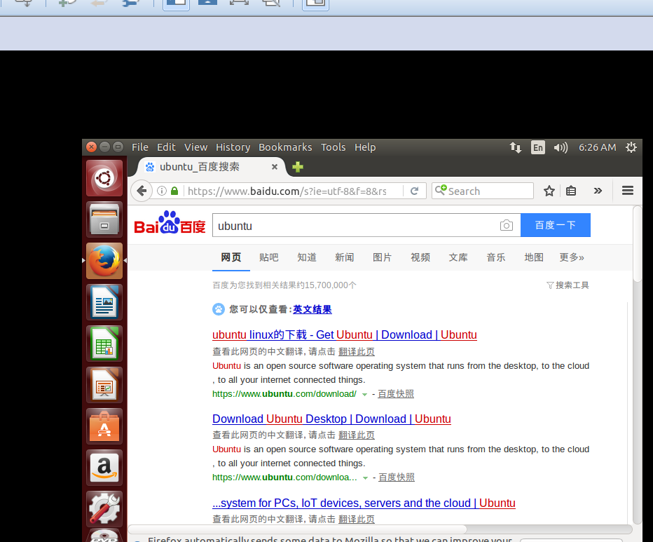
就能上网了

更新vmtools 就能在ubuntu里面设置分辨率了

ubuntu 使用方法.按键盘win 建,输入t ,就会出现terminal ,把他拖到左边的快捷栏里面,打开后,屏幕左上角有edit,perform设置字体.带图形界面的linux就是简单多了.

 

继续装软件:

java:https://www.linuxidc.com/Linux/2015-01/112030.htm

 如何用root来登录图形界面.从而随便复制粘贴.

在网上看了n种办法，问题是我的ubuntu根本没有system——>preferences——>……啥的

最后终于搞定。



安装ubuntu时输入的用户名和密码不是root，只是一个普通用户，连个文件夹都新建不了。



首先启动root

$ sudo passwd root

输入你希望的root密码

然后

$ su

# vim /etc/lightdm/lightdm.conf

# o //进入编辑模式

最后一行输入 greeter-show-manual-login=true

按 esc按钮

输入 :wq //保存并退出


修改后为：

[SeatDefaults]

greeter-session=unity-greeter

user-session=ubuntu

greeter-show-manual-login=true

重启机器

登录界面就可以选择用户了，登陆root即可。




之后,shudown里面选restart,开启周出现一个login用户,在里面输入root,
然后输入密码.进去就是root图形账号.!!!!!!

View Code

多用户注意点:

装环境一定要先切用户,各个用户之间的环境不共享!!!

 

 

 

 

---

 spyder设置默认模板:

tools-preference-editor-advance

 

---

 

https://www.cnblogs.com/wubdut/                 斌哥的博客---吴斌

 

---

 

django

1.pip install django  

2.开启vs2017

3.新建项目-python-web项目-django

https://www.cnblogs.com/feixuelove1009/p/5823135.html   (注意这里面的区别,views 在vs2017中是在app文件夹里面的)

4.写好后,项目上启动cmd 输入 python manage.py runserver 127.0.0.1:8000

5.浏览器　　http://127.0.0.1:8000/index/

注:.用proxifier 中设置代理规则,里面的输入127.0.0.1:65535,规则direct即可.就不会被proxifier改代理上不去这个网了.

6.安装django的需要版本：https://www.cnblogs.com/ld1226/p/6637998.html

教程：https://docs.djangoproject.com/en/2.0/intro/tutorial01/

 参考:https://www.cnblogs.com/feixuelove1009/p/5823135.html

---

 

win10激活

http://www.xitongzhijia.net/soft/79575.html        关闭防火墙,然后激活就成功了

 

---

 

解决vs2017和proxifier的冲突.

把python anaconda里面的程序python.exe. pythonw.exe都放到proxifier的列表里面设置direct直连即可.

 

---

 

如何不用pycharm来建立python的一些项目:比如scrapy        (pycharm要的配置太高)

我还是用vs2017,比spyder强大多了.调试更详细

如何用vs2017建立vs2017没有模板的项目:

1.d盘建立一个目录叫爬虫练习

2.在目录里面开powershell或者cmd  输入 scrapy startproject ArticleSpider

3.启动vs2017 , 点文件-新建-项目-python- 从现有的python代码-文件夹选择上面的爬虫练习文件夹-确定-下一步-完成  即可.自动把文件夹变成项目了.

 

---

 

网易云课堂:

linux 高级系统管理: 技术LVM:逻辑卷

软件测试:V模型,W模型,回归测试,冒烟测试,alpha,beta,pareto原则(8,2原则)

黑盒:等价类划分法,边界值法,因果图,正交表,场景法

什么事正交表:(1)每一列中，不同的数字出现的次数是相等的。(2)任意两列中数字的排列方式齐全而且均衡 !也就是说只是考虑2个因素的全排列.而不考虑全部的n排列.

所以一个3因素*2特征的实验需要 4行即可.怎么算的? 

白盒:逻辑覆盖,判定覆盖,语句覆盖

圈的复杂度:边-节点数+2=把平面分成几个区域

 

linux命令:

umask 设置创建的默认权限 (为什么叫这个,因为User's Mask  默认权限就是一个面具)

chattr lsattr 设置,查看权限　　set_uid:chmod u+s  xxx # 设置setuid权限

ln -s  /tmp/yum.log /root/111/yum.log 创立软连接. (注:如果你用软连接时候写的不是绝对路径,那么移动文件之后,可能会bug找不到源文件)  

注:ln -s 命令先写主文件目录,后写小的软文件目录

硬连接:不能对目录做,他是用anode来存储的.删除一个,另一个无所谓.硬连接也不能跨分区

ls -i   就能看文件的anode了.他就是文件的本质存储的位置

---

 

软连接非常实用的一个技术:磁盘文件的一种移动扩容方法.!!!!!!!

比如/boot/aming.log 这个目录/boot已经满了,/root 里面还很大,  但是我还是要往这个/boot地址写入,那么用软连接来实现这个功能

cp /boot/aming.log /root/aming.log

rm /boot/aming.log

ln -s /root/aming.log /boot/aming.log

只需要这3行命令就够了.非常牛逼,当然也可以用上面的LVM技术对逻辑分区扩容

 

---

 https://ke.qq.com/webcourse/index.html#cid=200566&term_id=100237673&taid=1277907389583222&vid=c1412o4kuqj

讲的非常好的操作系统课程.

跟io有关的就一定跟阻塞太有关,否则无关.

 

变量自加,自减需要利用寄存器.所以翻译成机器语言是都3句话.

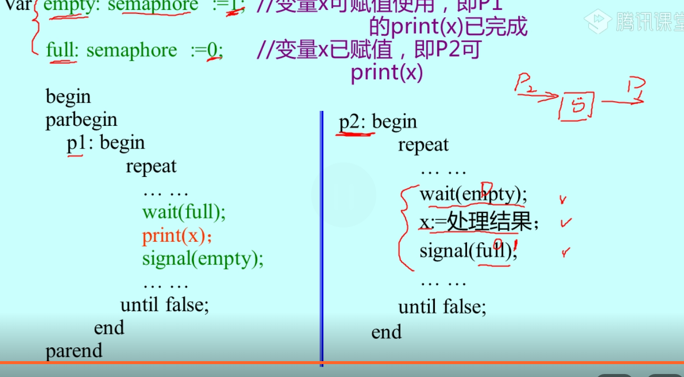
 记录型信号量的使用:

 

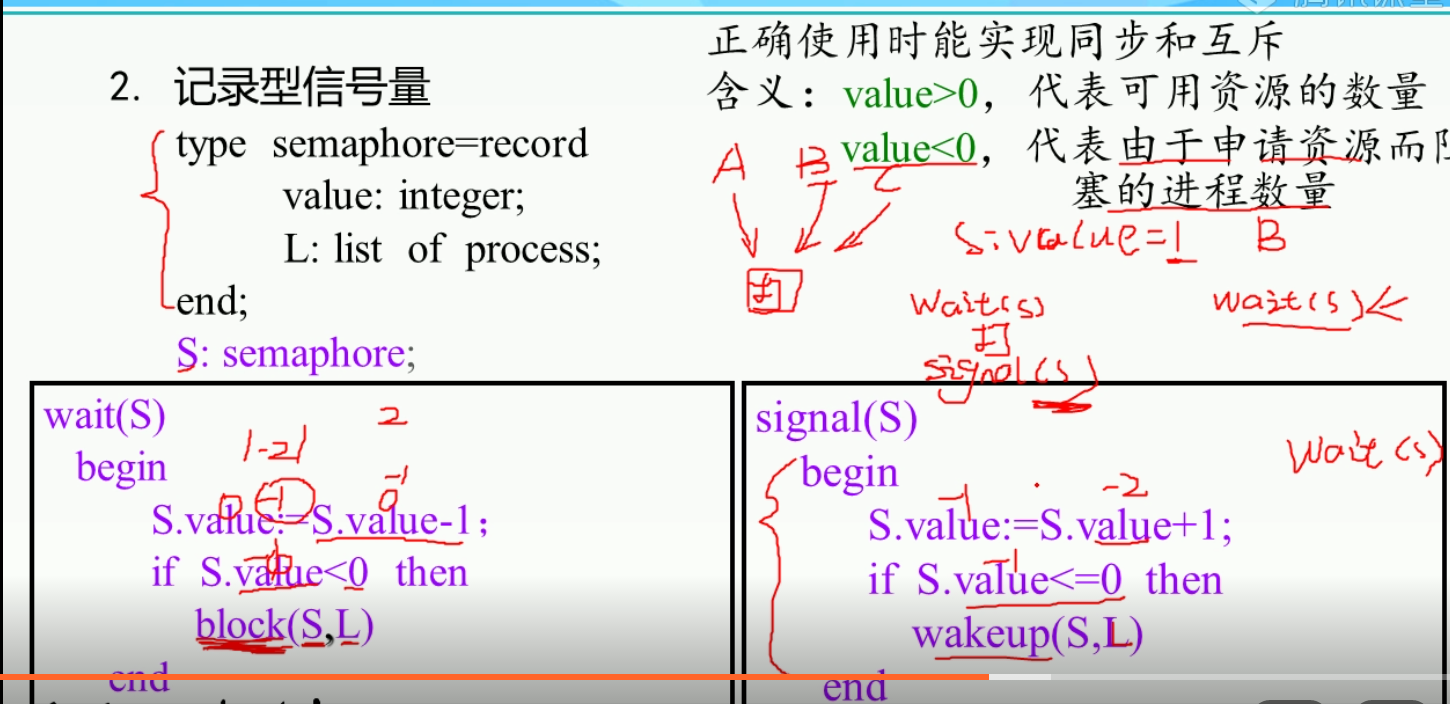
这个记录型信号量非常有用:例子:

一个打印机,两个工作a,b

信号量是打印机这个资源的一个描述.

记作typer,他的属性一个value=1(2个打印机就初始化为2),一个L=[],方法一个wait,一个signal ,

a先进来,一个进程进来,打印就就运行wait函数.这样信号量value变成0了.因为0不小于0所以a直接运行不用等.

b这时候才进来,还是运行wait函数,这时候value就变成-1了,所以触发block函数.b进入L中

这时候a打印完了,他出来,触发signal函数.value变成0,触发wakeup函数.所以b从队列中弹出.

这时候b可以进入了,并且不用wait函数.b直接运行.

这时候a又要打印,所以typer又进入wait函数.value变成-1,a进入队列等待.整个过程完美的实现了临街资源同一时间只能被一个进程访问.

(总结:进程从外界进入打印机就调用wait函数     进程是被wakeup唤醒的就直接运行!!!!!!!    进程运行完毕调用signal函数)

 

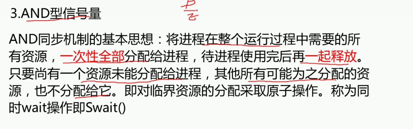
对上面的信号量作用到多个共享资源时候发生的死锁现象,继续做优化.就是下面的and型信号量

1.互斥

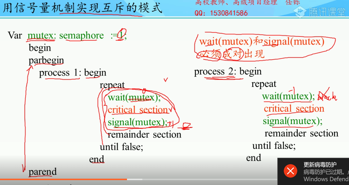
2.前驱:

 

3.合作,同时

 

 

 

 

---

 

 

云计算课程:

https://ke.qq.com/webcourse/index.html#course_id=269104&term_id=100317753&taid=1945925128035120&vid=y1423459vg1

 

---

 

马哥linux 讲bash脚本

http://study.163.com/course/courseLearn.htm?courseId=712012#/learn/video?lessonId=876097&courseId=712012

讲的很细

#!/bin/bash
groupadd -g 8008 newgroup
useradd -u 3006 -G 8008 mage   #-g ,-u 表示的是id号
#可以传入位置参数了
lines=$(wc -l $1|cut -d ' ': -f1)
echo $1 has $lines lines.
#useradd $1
echo $1|passwd --stdin$1 &>/dev/null #把echo出来的东西用--stdin 给passwd &>把错误信息给删除了.

for userno in `seq 301 310`
do
　　useradd user${userno}
done

dest=/tmp/dir-$(date+%Y%m%d-%H%M%S)
mkdir $dest
for i in {1..10}
do 
   touch $dest/file$i
done

#变量的运算用let
num1=9
num2=9
let num1+=9  #这就方便多了
#算数运算不赋值
echo $[$num1+$num2]    #这里面的第一个$表示算数运算符,第二第三个表示取变量值
#expr
echi "the sum is `expr $num1 + $num2`"    #第一要用`号,第二要注意+号左右带空格

#获取所有的user_id:
for  i in `cut -d: -f3 /etc/passwd`
do 
   echo $i
done

#传入一堆地址,返回地址内文件个数 ,$*可以把一堆变量当一个list传入
for file in $*
do 
   echo file
done


#添加用户:
if [ $# -lt 1 ]; then 
   exit 2
fi


if  ! id $username &>/dev/null ; then
    useradd $username
fi
#返回任意多个参数的嘴大值
max=0
for i in $*
do 
   if [ $max -lt $i ]; then 
          max=$i
   fi
done
#看一个文件是否存在空白行:
if grep "^[[ :space ]]*" $1; then
   echo '$1 has $(grep "^[[ :space ]]*" $1 |wc -l ) blank lines.' 
fi
#改主机名:
if [ -z '$localhost' -o '$localhost'=='localhost' ]; then
    localhost magedu.cn
fi

#创建1个文件
for i in `seq 1 10`; do    echo   $i>>1.txt; done

 

 AWK高级应用:

awk 'NR==1' 1.txt            返回第一行

awk 'END{print $0}'  1.txt    打印最后一行

 

---

 

 

python 连接mysql: pymysql 基本命令:       这个mysql浏览器输入127.0.0.1:3306 是没用的.只能用下面的py脚本连接

pymysql基本方法:

View Code

---

ccna网络精品课程:

http://study.163.com/course/courseLearn.htm?courseId=1003605098#/learn/video?lessonId=1004115689&courseId=1003605098

局域网用交换机连

广域网用路由器连

上来ping 127.0.0.1 来看网卡是不是好的. 所以127就给操作系统了

ip   子网掩码     网络位    主机位

 有效的子网掩码的范围 到/30

vrsm :利用子网掩码再划分来吧网络继续分割

 

 

 

---

 

huffman编码:

给一个字符串aabbccde对他进行huffman编码

a频率2

b频率2

c频率2

d频率1

e频率1

那么需要5个节点.结论:每一个编码都可以表示成每个非叶子节点恰好有2个子节点的2茶树,树的边上左写1右写0.

那么叶子节点表示成根到叶子的编码就是要的码

1.画树  2.给编码    3.按照频率大的给短的编码即可.但是树的构造需要技巧才能让最后的码最短

使用哈夫曼编码来编码字符串"aaaabbcd"时，得到的编码长度为多少?

 

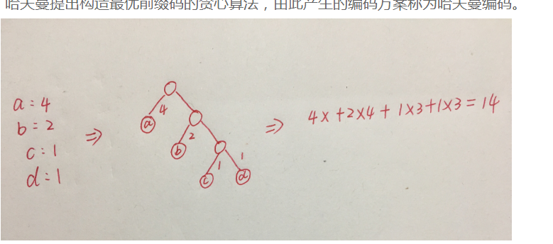
如果写成平衡树就需要16个,非平衡树就14个.这个也是分问题的

比如对abcd编码,用平衡树就更短.这个需要试.

---

 计算机题目:

递归函数最终会结束，那么这个函数一定？

有一个分支不调用自身
采用递归方式对顺序表进行快速排序，下列关于递归次数的叙述中，正确的是（）

递归次数与每次划分后得到的分区处理顺序无关
对递归程序的优化的一般的手段为（）   牛逼的例子.这样栈里面的元素永远大o1

以斐波那契数列为例子
普通的递归版本
int fab(int n){
    if(n<3)
        return 1;
    else
        return fab(n-1)+fab(n-2);  
}

具有"线性迭代过程"特性的递归---尾递归过程
int fab(int n,int b1=1,int b2=1,int c=3){
    if(n<3)
        return 1;
    else {
        if(n==c)
             return b1+b2;
        else
             return fab1(n,b2,b1+b2,c+1);
    }
}
以fab(4)为例子
普通递归fab(4)=fab(3)+fab(2)=fab(2)+fab(1)+fab(2)=3  6次调用
尾递归fab(4,1,1,3)=fab(4,1,2,4)=1+2=3                         2次调用

View Code

下列方法中，____不可以用来程序调优？

使用多线程的方式提高 I/O 密集型操作的效率
IO密集型表示大部分情况下IO处于繁忙状态。多线程适合于CPU等待长时间IO操作的情况，比如网络连接数据流的读写
。在IO密集型情况下IO操作都比较慢，因此需要专门开线程等待IO响应，而不影响非IO任务的执行。
递归函数中的形参是（）

自动变量

在间址周期中，______。

对于存储器间接寻址或寄存器间接寻址的指令，它们的操作是不同的

下列哪一个是析构函数的特征（）

一个类中只能定义一个析构函数
标准ASCII编码是（）位编码。

7

位操作运算符:参与运算的量，按二进制位进行运算。包括位与(&)、位或(|)、位非(~)、位异或(^)、左移(<<)、右移(>>)六种。
浮点数可以做逻辑运算,但是不能做位运算.

&&：逻辑与，前后条件同时满足表达式为真
||：逻辑或，前后条件只要有一个满足表达式为真
&：按位与
|：按位或
&&和||是逻辑运算，&与|是位运算

以下关于过拟合和欠拟合说法正确的是

过拟合可以通过减少变量来缓解

两台主机A和B已建立了TCP连接，A始终以MSS=1KB大小的段发送数据，并一直有数据发送；B每收到一个数据段都会发出一个接收窗口为9KB的确认段。

若A在T时刻发生超时时拥塞窗口为8KB，则从T时刻起，不再发生超时的情况下，经过10个RTT后，A的发送窗口是 （）

9KB
在Linux系统中，因为某些原因造成了一些进程变成孤儿进程，那么这些孤儿进程会被以下哪一个系统进程接管？

init
在软件开发中，经典的模型就是瀑布模型，下列关于瀑布模型的说法正确的是()

瀑布模型采用结构化的分析与设计方法，将逻辑实现与物理实现分开

 

---

深度学习:
维数灾难是什么:当特征特别多的时候,维数变高,样本数量相对会不够用.分类后的空间占整个空间变小.繁华能力变差.
https://ke.qq.com/webcourse/index.html#course_id=240557&term_id=100283770&taid=1552484648856493&vid=i1421vqqhew
推荐系统:
视频学的不多,还是要从书上基础来补.统计概率,机器学习,深度学习.这些.
https://ke.qq.com/webcourse/index.html#course_id=277276&term_id=100328034&taid=1988093116955420&vid=v1424iibikr
深度学习优化:
1.损失函数,替代损失函数.比如交叉熵来替换准确率来分类.

---

复习概率,用于给数据一顿分析.
●贝叶斯

     

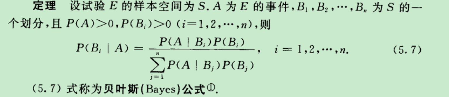
     理解就是左边是一个分类问题的概率.我们已经知道了A这个事件发生了,也就是A这个物体的符合这个特征已经知道了.那么他属于Bi这个类的概率是多少?

      理解右边公式:分子就是P(A交B)而已.分母就是全概率公式呗表示P(A) 两个一除,显然表示当A已经发生了的时候再发生Bi的概率,也就是条件概率.证毕.

　　应用:朴素贝叶斯也就是上面说的A的特征已经知道了.求A属于Bi类的概率.朴素贝叶斯说的是各个条件之见的影响是没有的.也就是概率上独立.

       A的特征是a1,...an   则P(A|Bi) =P(a1|Bi)*...*P(an|Bi)    也看做极大似然.道理都一样.感觉统计学思想本质就是一个极大似然.说一堆其实化简化简都一个.

　　然后我们的P(aj|Bi)这个概率是通过经验或者train集来获得的.获得方法count即可.(看Bi类里面属性为aj的有多少,然后除一下Bi里面元素个数)

●分布: 0-1分布, 伯努利试验(二项分布,也就是多重0-1分布), 

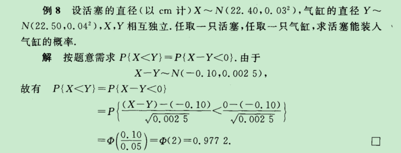
  连续分布: 均匀分布,指数分布(无记忆性),正态分布(3sigma: 1:68  2:95.4 3: 99.7) 标准正态分布:φ(-x)=1-φ(x)

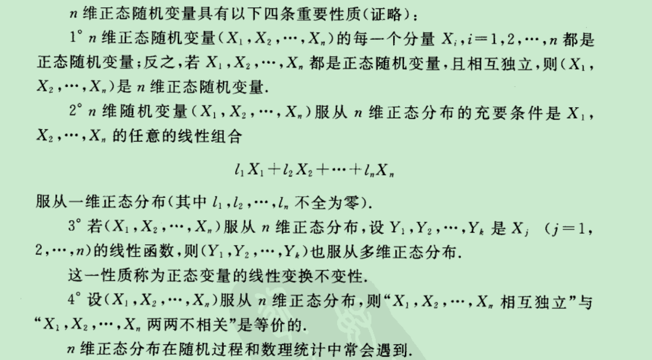
  2维正太分布的边缘分布与参数rho 无关,所以可以证明:单由一个分布的边缘分布是不能决定这个分布的联合分布的.

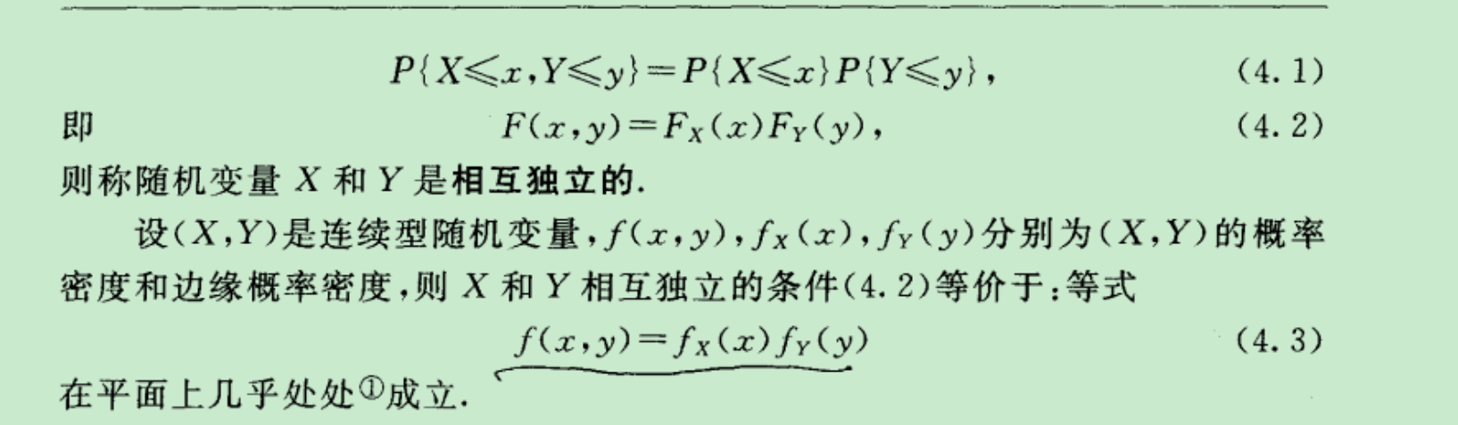
分布概率独立=独立=边缘概率独立 (证明显然)

 

核心定理:怎么证明?

往证: F(h,g)=F(h,.)*F(.,g)

左边=sigma所有x的取值,y的取值s.t.h=h1且g=g1的取值 

右边=(sigma 所有x的取值取s.t.h=h1) (sigma y的取值s.t.g=g1)  利用假设证毕.

●期望：设离散型随机变量的分布是P{X=xk}=pk  ，那么如果级数∑xkpk绝对收敛，那么他就定义为随机变量X的数学期望。

为什么这么要求绝对收敛而不是收敛。

1/2 - 1/3 + 1/4 - 1/5 + 。。。就是条件收敛。算他的和是几：
设X=1/2 - 1/3 + 1/4 - 1/5 + 。。。   他是ln（1+x）的泰勒展开式所以他等于1-ln（2）=0.306，我们说他是期望的话，给X一个概率分布，设成正太吧
，把正太的区间概率值都给这个区间内的1/n ，即可。即假设级数∑xkpk，的每一项xkpk=1/n乘以正负号。但是这显然不能说明n趋紧无穷的时候X这个取值趋近于0.306，因为显然后面无穷
多项都趋近于0的。这个跟常识矛盾，所以要加入绝对收敛这个条件。

 ●重要题型：

 

 

●样本的4个分位数, 箱线图,  修正箱线图,  我们采用中位数来描述数据的中心趋势,因为他比平均数更不受异常值干扰.

●常用计算公式:

标准正态分布密度函数: 

D(X)=E(X^2)-E(X)^2              (方差=先平方再期望-先期望再平方)

E(X^4)=3

证明:

http://blog.sina.com.cn/s/blog_4cb6ee6c0102xh17.html

所以卡方分布自由度为n:期望是n,方差是2n

●点估计:

样本均值=(x1+...+xn)/n     样本方差:sum(xi-x平均)/(n-1)

●极大似然估计:

设x1,...,xn 是样本值, 概率密度函数是f(x,θ). 

那么答案是θ 取值使得Πf(x,θ) 最大即可. 事实上更常用的是求左面式子取ln后的极值. (因为乘机爆炸问题)

●评价估计量:

无偏性,有效性,相合性.

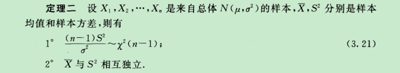
●正太分布的抽样的均值和方差的分布:

 

 

 所以有这个非常重要的公式:  最重要的公式!

上面是最核心的公式:解释:Xi是你观察一个独立重复时间的发生频率.那么用上式可以刻画μ和σ.

中心极限定理:一个完全相同的实验重复无穷次.那么观测值的平均值是一个正态分布.

统计学2个方法;1.估计  2.假设检验

假设检验例子:

  

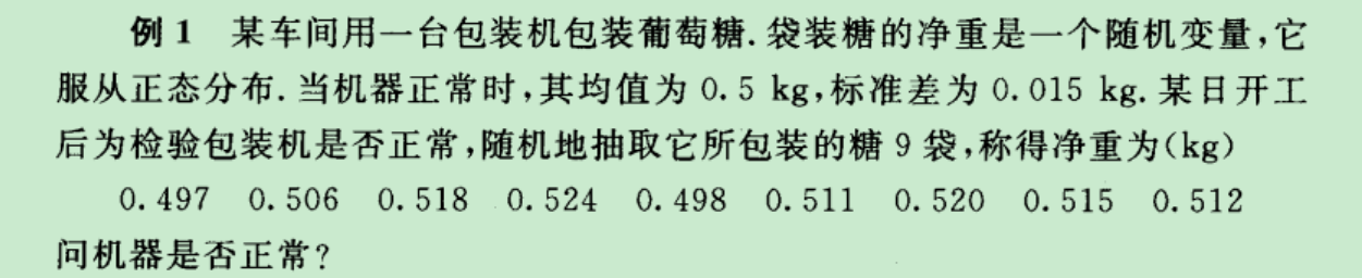
解答:首先套用最重要的公式.知道(xhat-miu0)/(σ/sqrt(n)) 是一个正态分布.假设检验成立,那么左边这个东西的取值不可能高于1.96,因为如果他高于1.96说明

miu为0.5这个条件触发了小概率事件.所以不对.(小概率时间认为不发生).拒绝域是均值过大,或者过小.所以是双边的拒绝域.即用0.025.

题目都很类似:继续套用一个题目:

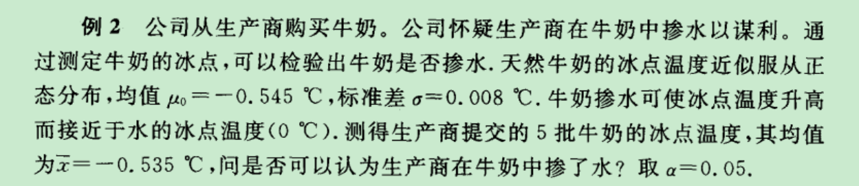
第一步:重要定理又来了:  (xhat-μ0)/(sigma/sqrt(n)) =标准正态分布

假设没有参水,那么上面正态分布就一定小于z(0.05).因为拒绝域是参水了,只可能往里面放水,只能让冰点提高,不能降低.所以预测

出来的只能是是否超过上0.05分点.所以比较上面的数根z(0.05)即可.超过就说明冰点变高了.说明参水了.

 

实际中:用的是t检验

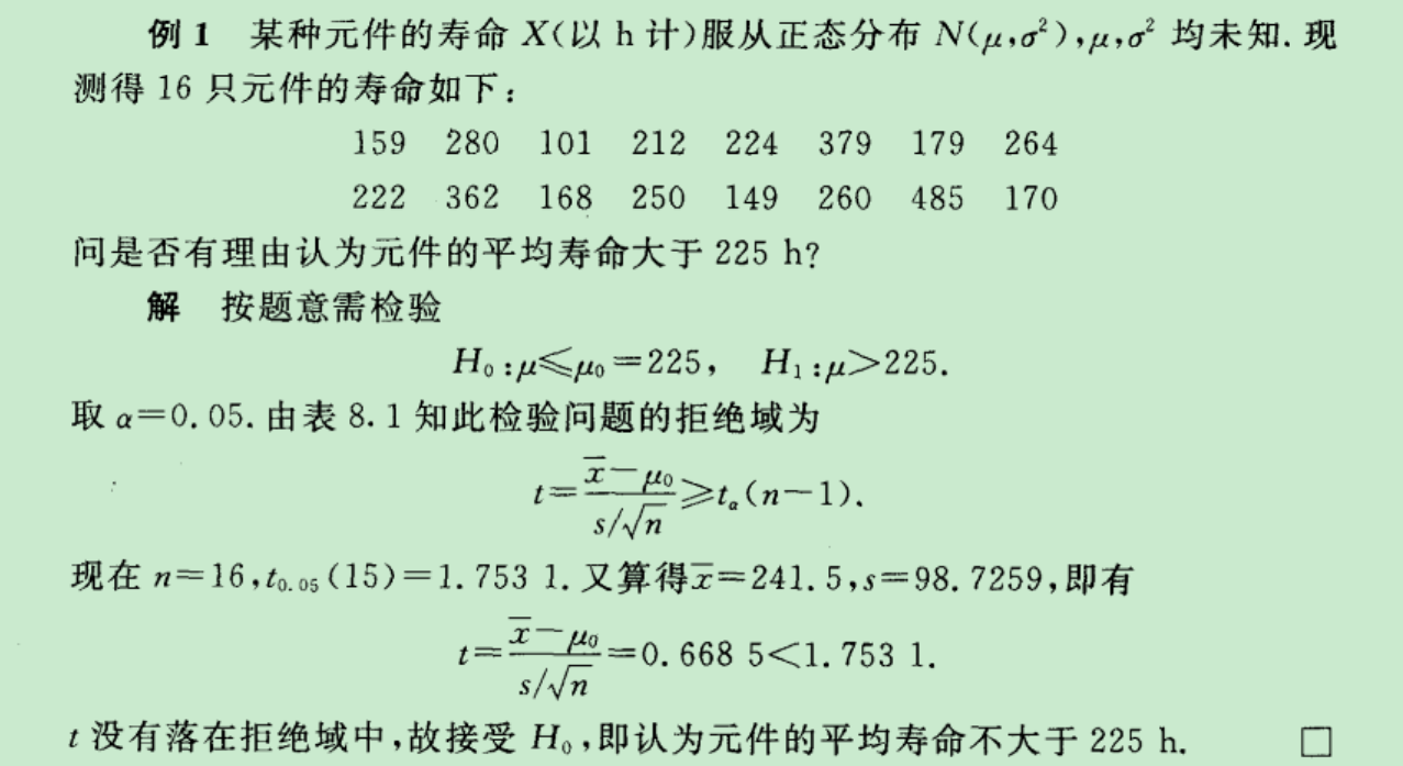
解释:就是用S来替代sigma就得到了t检验.拒绝域是零件寿命过小.所以是单边拒绝域.所以直接带入t(0.05)(n-1)即可.

●验证方差:用卡房检验.

●分布拟合检验:当分布不知道的时候

 

随机过程:加入时间变量的分布就是随机过程了.

刻画:均值函数,相关函数,协方差函数.

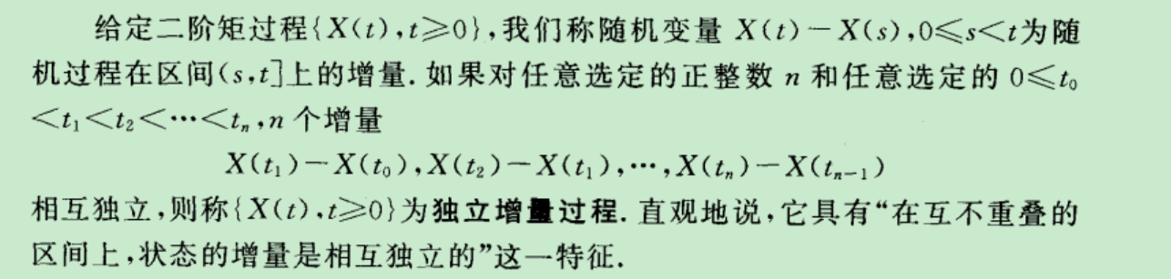
马尔科夫过程定义:

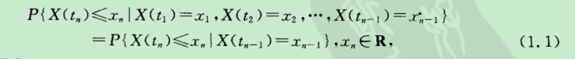
独立增量过程定义: 就是时间不重叠的部分,差分,独立

 

 应用时间序列分析:王燕:

1.描述性分析:通过画图,看出规律  (是对时间序列分析必须的一步)

2.统计学方法:1.谱分析:就是用sin,cos级数组合来逼近任意一个函数.

 　　　　　　2.时域分析:也就是一个时间是他之前的一段时间的取值的函数.

3.做假设检验来吧序列归类.

　　1.平稳时间序列:如果序列有趋势性或者周期性,他就不是平稳序列.自相关系数下降速度很快就是,并且没有周期性.

　　2.纯随机性检验:Q统计量.是纯随机性的一定是平稳的时间序列.所以一般也不用检验了.看一眼上面第一条就行了.

4.方法性工具:

　　1.p阶差分和k步差分.(我很好奇,为啥不用比分.就是t时刻数据/t-1时刻的数据)

5.平稳时间序列分析:ARMA

　　说白了就是仿射函数.

　　1.判定模型的平稳性:看图像法,特征根法,平稳域(也就是用特征根来算的)

　　2.平稳性和可逆性条件.

　　3.建模调参即可.

6.非平稳:

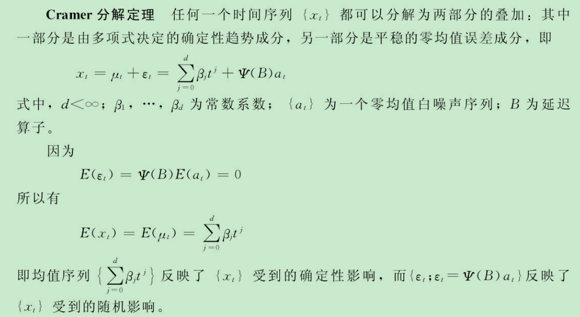
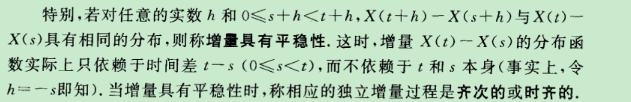
这不就是lagrange定理么,多项式逼近任何函数,然后加一个误差函数e.核心就是算这个多项式.

数据预处理的方法:

1.趋势分析:线性拟合,曲线拟合.(都是out的方法,怎么可能这么简单的函数就拟合了!!!!!!!!!!!!!!!!!!!!!!!!!!!!!!!!!!!!!!!!!!!!!!!!!没卵用)

2.数据平滑法:移动平滑法, n期移动平均,指数平滑法,holt平滑法(都没乱用!!!!!!!!!!!!)

3.季节分析

4.X-11方法

 随机分析方法:

1.线性趋势:用1阶差分

2.曲线趋势:用2阶

3.固定周期的序列:进行周期步长的周期差分

 

 

 

 

 

 

 

 

 

 

 

---

 

去除pdf的安全和加密:

http://www.liangchan.net/soft/softdown.asp?softid=8065

下载后跑一下即可.

 

 

 

 

 

 

 

 

---

 深度网络好文章:

 https://blog.csdn.net/u014696921/article/details/52768311　  

 

---

 

sqlite3的使用:
●python自带,直接cmd里面输入sqlite3就进入了

---

发现拔罐子祛痘祛湿效果很好,但是不能把时间长,容易起水泡

---

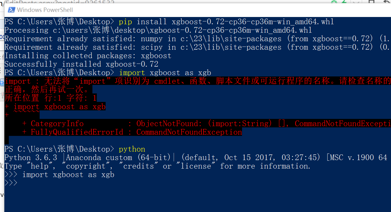
2018-07-31,15点08 学习xgboost
●复习决策树:
划分的依据:信息熵增益比(本质就是各个分类的纯度越来越高)
●回归树:就是算方差,越小越好.最后生成的是分段的常函数.
 举个例子:拟合(1,2)  (3,4) (5,10) 这3个点.那么就有2个分点,第一个分店是(1+3)/2  第二个是(3+5)/2 
第一个分店算完方差是0+(4-7)^2/2+(10-7)^2/2=9  第二个分店:是1所以选第二个分店也就是4.小于4用3来画,大于4用10来画.
图案就是

逼近效果还可以.能比线性回归好一点.

    ●xgboost就是改loss function 改成 mse+叶子结点个数+叶子节点的数值 就是这3个部分了.(mse也就是上面回归树说的方差:因为预测值取的就是平均数)

实际使用xgboost:

https://blog.csdn.net/flydreamforever/article/details/70767818 按照步骤安装成功.

 实例:

分类

from sklearn.datasets import load_iris
import xgboost as xgb
from xgboost import plot_importance
from matplotlib import pyplot as plt
from sklearn.model_selection import train_test_split

# read in the iris data
iris = load_iris()
print(iris)

X = iris.data
y = iris.target

X_train, X_test, y_train, y_test = train_test_split(X, y, test_size=0.2, random_state=0)

# 训练模型
'''
学习xgboost的使用:
在这里可以查询函数的含义:
http://xgboost.apachecn.org/cn/latest/python/python_api.html?highlight=n_estimators
下面是分类器的参数说明:
max_depth:每个树的高度
objective:是一个重要的函数,可以自己定义.这里面是多分类softmax
'''
model = xgb.XGBClassifier(max_depth=50, learning_rate=0.01, n_estimators=16000, 
                          silent=True, objective='multi:softmax')
model.fit(X_train, y_train)

# 对测试集进行预测
ans = model.predict(X_test)

# 计算准确率
cnt1 = 0
cnt2 = 0
for i in range(len(y_test)):
    if ans[i] == y_test[i]:
        cnt1 += 1
    else:
        cnt2 += 1

print("Accuracy: %.2f %% " % (100 * cnt1 / (cnt1 + cnt2)))

# 显示重要特征
plot_importance(model)
plt.show()

View Code

回归:

 

# -*- coding: utf-8 -*-
"""
Created on Fri Jul 20 10:58:02 2018


@author: 张博
"""

#读取csv最稳的方法:
#f = open(r'C:\Users\张博\Desktop\展示\old.csv')
#data = read_csv(f,header=None)





'''
画图模板:
from matplotlib import pyplot
data=[]
pyplot.plot(data,color='black')
pyplot.show()

'''



'''
获取当前时间:
import datetime
nowTime=datetime.datetime.now().strftime('%Y-%m-%d %H:%M:%S')#现在
nowTime=((nowTime)[:-3])
print(nowTime)
'''


'''
写文件的模板
with open(r'c:/234/wucha.txt','w') as f:
      wucha=str(wucha)
      f.write(wucha)
'''



'''
手动加断电的方法:raise 
'''








# -*- coding: utf-8 -*-
"""
Created on Fri Jul 20 10:58:02 2018


@author: 张博
"""

#读取csv最稳的方法:
#f = open(r'C:\Users\张博\Desktop\展示\old.csv')
#data = read_csv(f,header=None)





'''
画图模板:
from matplotlib import pyplot
data=[]
pyplot.plot(data,color='black')
pyplot.show()

'''



'''
获取当前时间:
import datetime
nowTime=datetime.datetime.now().strftime('%Y-%m-%d %H:%M:%S')#现在
nowTime=((nowTime)[:-3])
print(nowTime)
'''


'''
写文件的模板
with open(r'c:/234/wucha.txt','w') as f:
      wucha=str(wucha)
      f.write(wucha)
'''



'''
手动加断电的方法:raise 
'''


# -*- coding: utf-8 -*-
"""
Created on Fri Jul 20 10:58:02 2018


@author: 张博
"""









# -*- coding: utf-8 -*-
"""
Created on Tue Jul 17 10:54:38 2018

@author: 张博
"""

# -*- coding: utf-8 -*-
"""
Created on Mon Jul 16 17:18:57 2018

@author: 张博
"""

# -*- coding: utf-8 -*-
"""
Spyder Editor

This is a temporary script file.
"""

#2018-07-23,22点54对学习率参数进行for循环来学习哪个最好RATE
for i in range((1)):
    
    import os
    os.environ['CUDA_VISIBLE_DEVICES'] = '0' #使用 GPU 0
    
    import tensorflow as tf
    from keras.backend.tensorflow_backend import set_session
    
    config = tf.ConfigProto()
    config.gpu_options.allocator_type = 'BFC' #A "Best-fit with coalescing" algorithm, simplified from a version of dlmalloc.
    config.gpu_options.per_process_gpu_memory_fraction = 1.
    config.gpu_options.allow_growth = True
    set_session(tf.Session(config=config))
    
    
    
    
    
    
    
    
    #老外的教程:非常详细,最后的多变量,多step模型应该是最终实际应用最好的模型了.也就是这个.py文件写的内容
    #https://machinelearningmastery.com/multivariate-time-series-forecasting-lstms-keras/
    
    '''
    SUPER_PARAMETER:一般代码习惯把超参数写最开始位置,方便修改和查找
    '''
    EPOCH=100
    LOOK_BACK=1
    n_features = 3         #这个问题里面这个参数不用动,因为只有2个变量
    RATE=0.55
    shenjing=62
    n_hours = LOOK_BACK
    
    
    
    
    
    import pandas as pd
    
    from pandas import read_csv
    from datetime import datetime
    # load data
    def parse(x):
        return datetime.strptime(x, '%Y %m %d %H')
    data = read_csv(r'E:\output_nonghang\out2new.csv')
    
    #应该把DD给删了,天数没用
    #切片和concat即可
    
    
    tmp1=data.iloc[:,2:3]
    tmp2=data.iloc[:,3]
    tmp3=data.iloc[:,1]

    data.to_csv('c:/234/out00000.csv')
    
#    for i in range(len(tmp3)):
#        if tmp3[i] in range(12,13):
#            tmp3[i]=1
#        if tmp3[i] in range(13,14):
#            tmp3[i]=2
#        else:
#            tmp3[i]=0


    #加一个预处理判断.判断数据奇异的点.
    #方法是:遍历一遍整个数据,如果这个点的数据比同时工作日或者周末的情况的mean的0.2还低
    #就说明这个点错了.用上面同比情况mean来替代.
    #2018-07-25,21点52跑出来百分之5.8错误率,说明这个修正的初始化过程非常重要!!不然就在
    #8左右徘徊.
    '''
    应该是更好的一种修改坏点的方法:
    比如7月23日3点的数据是错的.那么我们就用7月1日到7月23日2点的数据做训练,然后来预测7越23日3点的数据
    把这个7月23日3点预测到的数据当成真是数据来给7月23日3点.后面的坏点都同样处理.
    
    比如如果7月23日3点和4点数据都坏了.(也就是显然跟真实数据差很多,我的判断是比同期的数据0.4呗还低)
    那么我先预测3点的数据,然后把这个预测到的数据当真实值,4点的数据用上前面预测到的3点的值继续跑.来
    预测4点的值.这样就把3,4点的值都修正过来了.当然时间上会很慢,比下面使用的平均数替代法要多跑2次深度学习.
    '''

    for i in range(len(data)):
        hour=data.iloc[i]['HH']
        week=data.iloc[i]['week']
        tmp56=data.query('HH == '+str(hour) +' and '+ 'week=='+str(week)+' and '+'index!='+str(i))
        tmp_sum=tmp56['Sum'].mean()
        
        if data.iloc[i]['Sum']< tmp_sum *0.4:
            data.iloc[i]['Sum']=tmp_sum 
            print('修改了如下行,因为他是异常点')
            print(i)
            
            
    
    #修改完毕


    tmp1=data.iloc[:,2:3]
    tmp2=data.iloc[:,3]
    tmp3=data.iloc[:,1]















    









    
    
    data=pd.concat([tmp2,tmp3,tmp1],axis=1)
#    print(data)
    
    
    
    
    
    data.to_csv('c:/234/out00000.csv')
    
    
    #因为下面的模板是把预测值放在了第一列.所以对data先做一个变换.
    
    
    
    
    
    
    
    
    
    
    
    
    
    #data.to_csv('pollution.csv')
    
    
    
    
    
    
    from pandas import read_csv
    from matplotlib import pyplot
    # load dataset
    dataset = data
    values = dataset.values
    
    
    
    ## specify columns to plot
    #groups = [0, 1, 2, 3, 5, 6, 7]
    #i = 1
    
    
    from pandas import read_csv
    from matplotlib import pyplot
    # load dataset
    #dataset = read_csv('pollution.csv', header=0, index_col=0)
    ##print(dataset.head())
    #values = dataset.values
    # specify columns to plot
    #groups = [0, 1, 2, 3, 5, 6, 7]
    #i = 1
    # plot each column
    #pyplot.figure()
    #图中每一行是一个列数据的展现.所以一共有7个小图,对应7个列指标的变化.
    #for group in groups:
    #    pyplot.subplot(len(groups), 1, i)
    #    pyplot.plot(values[:, group])
    #    pyplot.title(dataset.columns[group], y=0.5, loc='right')
    #    i += 1
    ##pyplot.show()
    
    
    
    from math import sqrt
    from numpy import concatenate
    from matplotlib import pyplot
    from pandas import read_csv
    from pandas import DataFrame
    from pandas import concat
    from sklearn.preprocessing import MinMaxScaler
    from sklearn.preprocessing import LabelEncoder
    from sklearn.metrics import mean_squared_error
    from keras.models import Sequential
    from keras.layers import Dense
    from keras.layers import LSTM
    # load dataset
    
    
    # integer encode direction
    #把标签标准化而已.比如把1,23,5,7,7标准化之后就变成了0,1,2,3,3
    #print('values')
    #print(values[:5])
    #encoder = LabelEncoder()
    #values[:,4] = encoder.fit_transform(values[:,4])
    ## ensure all data is float
    #values = values.astype('float32')
    #print('values_after_endoding')
    #numpy 转pd
    import pandas as pd
    #pd.DataFrame(values).to_csv('values_after_endoding.csv')
    #从结果可以看出来encoder函数把这种catogorical的数据转化成了数值类型,
    #方便做回归.
    #print(values[:5])
    # normalize features,先正规化.
    
    
    
    
    #这里面系数多尝试(0,1) (-1,1) 或者用其他正则化方法.
    scaler = MinMaxScaler(feature_range=(-1, 1))
    scaled = scaler.fit_transform(values)
    print('正规化之后的数据')
    
    pd.DataFrame(scaled).to_csv('values_after_normalization.csv')
    
    # frame as supervised learning
    
    
    
    
    # convert series to supervised learning
    #n_in:之前的时间点读入多少,n_out:之后的时间点读入多少.
    #对于多变量,都是同时读入多少.为了方便,统一按嘴大的来.
    #print('测试shift函数')
    #
    #df = DataFrame(scaled)
    #print(df)      # 从测试看出来shift就是数据同时向下平移,或者向上平移.
    #print(df.shift(2))
    def series_to_supervised(data, n_in=1, n_out=1, dropnan=True):
        n_vars = 1 if type(data) is list else data.shape[1]
        df = DataFrame(data)
        cols, names = [],[]
        # input sequence (t-n, ... t-1)
        for i in range(n_in, 0, -1):
            cols.append(df.shift(i))
            names += [('var%d(时间:t-%s)' % (j+1, i)) for j in range(n_vars)]
        # forecast sequence (t, t+1, ... t+n)
        for i in range(0, n_out):
            cols.append(df.shift(-i))
            if i == 0:
                names += [('var%d(时间:t)' % (j+1)) for j in range(n_vars)]
            else:
                names += [('var%d(时间:t+%d)' % (j+1, i)) for j in range(n_vars)]
        # put it all together
        agg = concat(cols, axis=1)
        agg.columns = names
        # drop rows with NaN values
        if dropnan:
            agg.dropna(inplace=True)
        return agg
    
    
    
    
    
    
    
    
    
    
    
    
    
    
    
    
    
    
    
    
    #series_to_supervised函数把多变量时间序列的列拍好.
    
    reframed = series_to_supervised(scaled, LOOK_BACK, 1)
    
    # drop columns we don't want to predict
    #我们只需要预测var1(t)所以把后面的拍都扔了.
    
    help111=series_to_supervised(values, LOOK_BACK, 1)
    
    
    
    print('处理的数据集')
    print(help111)
    
    # split into train and test sets
    values = reframed.values
    n_train_hours = int(len(scaled)*0.75)
    train = values[:n_train_hours, :]
    test = values[n_train_hours:, :]
    # split into input and outputs
    n_obs = n_hours * n_features
    train_X, train_y = train[:, :n_obs], train[:, -n_features]
    test_X, test_y = test[:, :n_obs], test[:, -n_features]
    #print(train_X.shape, len(train_X), train_y.shape)
    #print(test_X.shape, len(test_X), test_y.shape)
    #print(train_X)
    #print(9999999999999999)
    #print(test_X)
    
    
    
    
    
    '''
    所以最后我们得到4个数据
    train_X
    train_Y
    test_X
    test_Y
    '''
    
    
    
    
    
    #下面我开始改成xgboost来跑
#    print(train_X.shape)
#    print(train_y.shape)
#    print(test_X.shape)
#    print(test_y.shape)
    
    
    
    '''
    Learning Task Parameters

Specify the learning task and the corresponding learning objective. The objective options are below:

objective [default=reg:linear]
reg:linear: linear regression
reg:logistic: logistic regression
binary:logistic: logistic regression for binary classification, output probability
binary:logitraw: logistic regression for binary classification, output score before logistic transformation
gpu:reg:linear, gpu:reg:logistic, gpu:binary:logistic, gpu:binary:logitraw: versions of the corresponding objective functions evaluated on the GPU; note that like the GPU histogram algorithm, they can only be used when the entire training session uses the same dataset
count:poisson –poisson regression for count data, output mean of poisson distribution
max_delta_step is set to 0.7 by default in poisson regression (used to safeguard optimization)
survival:cox: Cox regression for right censored survival time data (negative values are considered right censored). Note that predictions are returned on the hazard ratio scale (i.e., as HR = exp(marginal_prediction) in the proportional hazard function h(t) = h0(t) * HR).
multi:softmax: set XGBoost to do multiclass classification using the softmax objective, you also need to set num_class(number of classes)
multi:softprob: same as softmax, but output a vector of ndata * nclass, which can be further reshaped to ndata * nclass matrix. The result contains predicted probability of each data point belonging to each class.
rank:pairwise: set XGBoost to do ranking task by minimizing the pairwise loss
reg:gamma: gamma regression with log-link. Output is a mean of gamma distribution. It might be useful, e.g., for modeling insurance claims severity, or for any outcome that might be gamma-distributed.
reg:tweedie: Tweedie regression with log-link. It might be useful, e.g., for modeling total loss in insurance, or for any outcome that might be Tweedie-distributed.
base_score [default=0.5]
The initial prediction score of all instances, global bias
For sufficient number of iterations, changing this value will not have too much effect.
eval_metric [default according to objective]
Evaluation metrics for validation data, a default metric will be assigned according to objective (rmse for regression, and error for classification, mean average precision for ranking)
User can add multiple evaluation metrics. Python users: remember to pass the metrics in as list of parameters pairs instead of map, so that latter eval_metric won’t override previous one
The choices are listed below:
rmse: root mean square error
mae: mean absolute error
logloss: negative log-likelihood
error: Binary classification error rate. It is calculated as #(wrong cases)/#(all cases). For the predictions, the evaluation will regard the instances with prediction value larger than 0.5 as positive instances, and the others as negative instances.
error@t: a different than 0.5 binary classification threshold value could be specified by providing a numerical value through ‘t’.
merror: Multiclass classification error rate. It is calculated as #(wrong cases)/#(all cases).
mlogloss: Multiclass logloss.
auc: Area under the curve
ndcg: Normalized Discounted Cumulative Gain
map: Mean average precision
ndcg@n, map@n: ‘n’ can be assigned as an integer to cut off the top positions in the lists for evaluation.
ndcg-, map-, ndcg@n-, map@n-: In XGBoost, NDCG and MAP will evaluate the score of a list without any positive samples as 1. By adding “-” in the evaluation metric XGBoost will evaluate these score as 0 to be consistent under some conditions.
poisson-nloglik: negative log-likelihood for Poisson regression
gamma-nloglik: negative log-likelihood for gamma regression
cox-nloglik: negative partial log-likelihood for Cox proportional hazards regression
gamma-deviance: residual deviance for gamma regression
tweedie-nloglik: negative log-likelihood for Tweedie regression (at a specified value of the tweedie_variance_power parameter)
seed [default=0]
Random number seed.
    '''
    
    #回归

        
    model = xgb.XGBRegressor(max_depth=10, learning_rate=0.1,
                             n_estimators=1600, silent=True, objective='reg:linear')
    model.fit(train_X, train_y)
    
    # 对测试集进行预测
    ans = model.predict(test_X)
    yhat=ans
    # 显示重要特征
    import xgboost

    
    axx=plt.rcParams['figure.figsize'] = (20, 3)
     
    xgboost.plot_importance(model)
    
    plt.show() 
#    import graphviz
#    xgboost.plot_tree(model)
#    
#    plt.show()   
    
    
    
    
    
    
    
    
    
    
    test_X = test_X.reshape((test_X.shape[0], n_hours*n_features))
    # invert scaling for forecast
    
    
    
    import numpy as np
    yhat=yhat.reshape(len(yhat),1)
    print(yhat.shape)
    print(test_X[:, -(n_features-1):].shape)
    
    #因为之前的scale是对初始数据做scale的,inverse回去还需要把矩阵的型拼回去.
    inv_yhat = np.concatenate((yhat, test_X[:, -(n_features-1):]), axis=1)
    inv_yhat = scaler.inverse_transform(inv_yhat)
    inv_yhat = inv_yhat[:,0]#inverse完再把数据扣出来.多变量这个地方需要的操作要多点
    # invert scaling for actual
    
    
    
    test_y = test_y.reshape((len(test_y), 1))
    inv_y = concatenate((test_y, test_X[:, -(n_features-1):]), axis=1)
    inv_y = scaler.inverse_transform(inv_y)
    inv_y = inv_y[:,0]
    
    
    
    
    
    
    
    
    
    with open(r'c:/234/inv_y.txt','w') as f:
          inv_y1=str(inv_y)
          f.write(inv_y1)
    with open(r'c:/234/inv_yhat.txt','w') as f:
          inv_yhat1=str(inv_yhat)
          f.write(inv_yhat1)
    
    
    
    # calculate RMSE
    rmse = sqrt(mean_squared_error(inv_y, inv_yhat))
#    print('RATE:')
#    print(RATE)
    print('输出abs差百分比指标:')
    #这个污染指数还有0的.干扰非常大
    #print(inv_y.shape)
    #print(inv_yhat.shape)
    wucha=abs(inv_y-inv_yhat)/(inv_y)
    #print(wucha)
    '''
    下面把得到的abs百分比误差写到 文件里面
    '''

    #with open(r'c:/234/wucha.txt','w') as f:
    #      print(type(wucha))
    #      wucha2=list(wucha)
    #      wucha2=str(wucha2)
    #      f.write(wucha2)
    
    with open(r'c:/234/sumary.txt','a') as f:
          rate=str(RATE)
          f.write(rate+'，')
          shenjing=str(shenjing)
          f.write(shenjing)
          f.write(',')
          wucha2=wucha.mean()
          wucha2=str(wucha2)
          f.write(wucha2)
          f.write('.')
          f.write('\n')
    
    
    wucha=wucha.mean()
    print(wucha)
    
    
    
    inv_y=inv_y
    inv_yhat=inv_yhat
    
    #print('Test RMSE: %.3f' % rmse)
    import numpy as np
    
    from matplotlib import pyplot
    pyplot.rcParams['figure.figsize'] = (20, 3) # 设置figure_size尺寸
    
    pyplot.rcParams['image.cmap'] = 'gray' # 
    pyplot.plot(inv_y,color='black',linewidth = 0.7)
    pyplot.plot(inv_yhat     ,color='red',linewidth = 0.7)
    
    pyplot.show()
    
    
    
    
    
    
    
    
    
    
    
    
    
    
    
    
    
    
    
    
    
    
    
    '''
    获取当前时间:
    import datetime
    nowTime=datetime.datetime.now().strftime('%Y-%m-%d %H:%M:%S')#现在
    nowTime=((nowTime)[:-3])
    print(nowTime)
    '''
    
    
    '''
    写文件的模板
    with open(r'c:/234/wucha.txt','w') as f:
          wucha=str(wucha)
          f.write(wucha)
    '''
    
    
    
    
    
    
    '''
    手动加断电的方法:raise NameError #这种加断点方法靠谱
    '''
    
    '''
    画图模板:
    import numpy as np
    
    from matplotlib import pyplot
    pyplot.rcParams['figure.figsize'] = (20, 3) # 设置figure_size尺寸
    
    pyplot.rcParams['image.cmap'] = 'gray' # 
    pyplot.plot(inv_y,color='black',linewidth = 0.7)
    
    
    pyplot.show()
    
    
    '''
    
    #读取csv最稳的方法:
    #f = open(r'C:\Users\张博\Desktop\展示\old.csv')
    #data = read_csv(f,header=None)
    

View Code

 

---

●模型的评估
公式:a1,a2同分布,独立那么D(a1-a2)=2σ方  推导:D(a1-a2)=E(a1^2)-2E(a1a2)+E(a2^2)=利用独立性=2(E(a1^2)-E(a1)^2) 证毕
　　　　　　　　　　显然不能把a2换成a1,因为虽然同分布但是换成a1表示他们是严格相关的,而事实上,他们是独立的

    a1,a2独立那么E(a1a2)=E(a1)E(a2)  这个怎么理解?两个变量无关,那么a1a2
性能指标:
    2分问题:
　　  查准率precision 查全率 recall　　PR曲线
　　交叉验证的处理:
　　　　

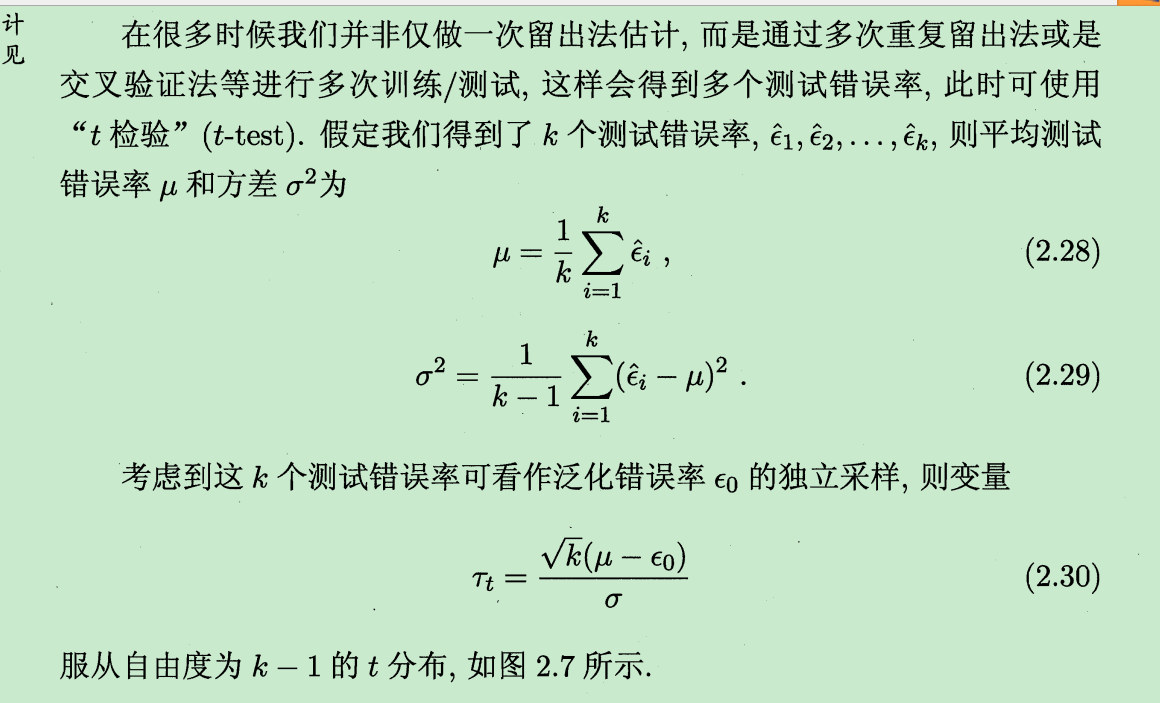
流程:假设错误率小于ε0,则计算后如果<t(k-1)0.05就可以说假设成立.

 

 

---

 

重学linux:
http://study.163.com/course/courseLearn.htm?courseId=956005&from=study#/learn/video?lessonId=1004214244&courseId=956005
ls -alh  方便查看文件大小
ls -d   看目录
--help  可以查询命令的使用方法.
复制粘贴: 鼠标中键
ll 命令 =ls -l
date -s 修改时间
date 查看时间
去掉锁屏:  https://blog.csdn.net/super828/article/details/79342862
定时开机的原理:用bios来启动
查看硬件信息:cat /proc/meminfo
动态查看日志:
tail -f /var/log/messages  这样只要文件俺动了,就能立即看到.
cp  /root/*.txt  /opt 把所有*.txt都复制过去.
!$ 表示上一个命令的参数
vim:/正想查找   数字+gg  调到那一行
账号信息:/etc/passwd   密码在 /etc/shadow

组账号信息:/etc/group  密码在  /etc/gshadow
直接改/etc/passwd里面 uid改成0 就变root了!
userdel -r [用户]  彻底删除,否则只删除passwd里面的对应行.
给用户密码: echo 123456|passwd -- stdin [用户]
取哈希: echo 123456|sha1sum
但是密码一样,在/etc/shadow 里面还是不一样.

chmod 修改权限  chmod u-w a.txt   chmod g+x a.txt   chmod o-r a.txt   chmod a=r a.txt (所有人)
ll -d test 看目录权限

chown san:bin  a.txt   修改所属主和所属组

拥有者没有w权限还是可以写:加!即可.
mount /dev/sr0 /mnt   挂载光盘
umount /mnt    取消挂载
rpm -ivh [软件包]
以来关系复杂就用 yum install   [软件包]
压缩:
对文本压缩比高,对图片和视频越压越大.因为他们已经压过了,再压反倒变大
file 文件类型的擦看
du [文件夹] 看文件夹的大小.
ps -aux
cat /proc 看参数
kill -9 [进程PID号]
killall
pstree
top -p [进程id号]   (-p 表示选id号)
看id号:   ps -aux |grep [进程名]
nice -n 5 vi a.txt   (设置进程的有限度)
renice -n 5 vi a.txt
grep -v 4 a.txt   -v表示取反
过滤空行 grep ^$ a.txt
find /etc/ name '*.txt'  查找名字是*.txt的文件

find /etc/ -perm 755  查找权限

find /etc/ -user 755  

find /etc/ -group 755  

---

C语言:http://study.163.com/course/courseLearn.htm?courseId=1004489035#/learn/video?lessonId=1048926708&courseId=1004489035

ide:Dev-C++ 用这个软件来做. 首先调试的设置方法:http://tieba.baidu.com/p/3976904106
太难用了,还是用vc6.0吧
跳动的小球:

//http://study.163.com/course/courseLearn.htm?courseId=1004489035&from=study#/learn/video?lessonId=1049009037&courseId=1004489035
//跳动的小球 
#include<math.h>
#include<stdlib.h>
#include<windows.h>
#include<stdio.h>
int main(void)
{
   int i ,j ;
   int x=10;
   int y=20;
   int velocity=1;
   int velocity2=1;
   while (1){ 
   if (x>10 ||x<0)
     velocity*=-1; //到边界的时候变向 
   if (y>20 ||y<0)
     velocity2*=-1; //到边界的时候变向 
   x=x+velocity;
   y=y+velocity2;
   for (i=0;i<x;i++)
      printf("\n");
   for (j=0;j<y;j++)
      printf(" ");
   printf("o\n");
   Sleep(50);
   
   system("cls");//这个函数能让屏幕清空,光标变回0,0位置 

   
   }
 } 
 
 
 
 
 
 
 
 
 
 /*
按F11开始编译和运行
 
默认需要输入的模板 
#include<math.h>
#include<stdio.h>
int main(void)
{

     printf("%d",x);
 } 

强转换:
x=(float)x3; 正确
x=float(x3); 正确
x5=(float)x5; 错误 因为转化类型后不能赋值给自己. 
读取字符:
scanf("%c %d",&b,&a); //键盘输入时候必须m 10213 
scanf("%c,%d",&b,&a); //键盘输入时候必须m,321 
scanf("%c%d",&b,&a); //键盘输入时候必须m 1023或者m 回车123 


for语句:
for (i=1;i<=n;i++)
  {s=s+i; 
  }

while语句:
while(i<=100)
{sum=sum+i;
} 

if语句: 

if (a<b) y=-1;
else if (x==0) y=0;
else y=1;

switch语句: 
switch (month)
{
case1: printf("January");break ;
case2: printf("Fanuary");break ;
default:printf("Fanuary");break ;
}










*/

View Code

飞机游戏:

//http://study.163.com/course/courseLearn.htm?courseId=1004489035&from=study#/learn/video?lessonId=1049009037&courseId=1004489035
//飞机游戏 
#include<math.h>
#include<stdlib.h>
#include<windows.h>
#include<conio.h>   //可以用getch() ;
 
#include<stdio.h>
int main(void)
{
   int i ,j ;
   int x,y=10;
   char input;
   char fired=0;
   int ny=15;//靶子的位置 
   int isKilled=0 ;
   while (1){ 
   system("cls");//这个函数能让屏幕清空,光标变回0,0位置 
   
   
   
   //靶子
   if (isKilled==0) {
   for (i=0;i<ny;i++)
      printf(" ");
   printf("+\n");}
   
   
   if (fired==0){
   for (i=0;i<x;i++)
      printf("\n");
   for (j=0;j<y;j++)
      printf(" ");
    printf("\n");}
   
   else
       {
           
   
   
   for (i=0;i<x+1;i++) //开枪时候多甩一行 
      {
          for (j=0;j<y;j++)
          {printf(" ");}
      
        printf("|\n");
      }
      
           if(y==ny){isKilled=1;} 
 
       fired=0;}
       
       
       
       
   //下面几行画飞机 
   for (j=0;j<y;j++)
          printf(" ");
   printf("o\n");//\n用于把光标甩到最左边 
   for (j=0;j<y-2;j++)
       printf(" ");
   printf("*****\n");
   for (j=0;j<y-2;j++)
       printf(" ");
   printf(" * * \n");
   //画完了 
   
   
   input=getch();//类似scanf会自动停住,好处是不用输入回车就能赋值了. 
   if (input=='s')
      x++;
   if (input=='w')
      x--;
   if (input=='a')
      y--;
   if (input=='d')
      y++;
   if (input==' ')
      fired=1;
   }
 } 
 
 
 
 
 
 
 
 
 
 /*
按F11开始编译和运行
 
默认需要输入的模板 
#include<math.h>
#include<stdio.h>
int main(void)
{

     printf("%d",x);
 } 

强转换:
x=(float)x3; 正确
x=float(x3); 正确
x5=(float)x5; 错误 因为转化类型后不能赋值给自己. 
读取字符:
scanf("%c %d",&b,&a); //键盘输入时候必须m 10213 
scanf("%c,%d",&b,&a); //键盘输入时候必须m,321 
scanf("%c%d",&b,&a); //键盘输入时候必须m 1023或者m 回车123 


for语句:
for (i=1;i<=n;i++)
  {s=s+i; 
  }

while语句:
while(i<=100)
{sum=sum+i;
} 

if语句: 

if (a<b) y=-1;
else if (x==0) y=0;
else y=1;

switch语句: 
switch (month)
{
case1: printf("January");break ;
case2: printf("Fanuary");break ;
default:printf("Fanuary");break ;
}










*/

View Code

 c语言的基础知识:

int a; 表示的是auto int a;他是一个自动类型变量,表示的是你不给他赋值他就是一个随机的(也叫狗屎值),他的生命周期是他所在的括号的范围内.

static int a;表示的是静态变量.不给他赋值他就自动表示的是0.

头文件:建立一个文件叫t2.h 然后cpp文件里面输入include "t2.h" 即可引入这个文件.

宏定义的使用:#define Pi 3.14156  
函数传递的是形参,不会对原来的进行修改,但是参数是数组的情况下就不是形参而是实参,因为他传递的是地址!
指针初始化一定要赋值 int *p=NULL 否则他会随机指向一个地方,不安全.
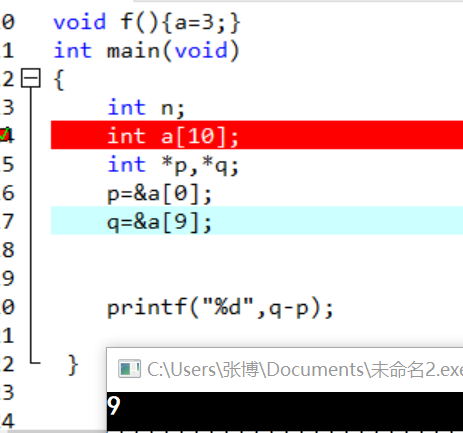
指针可以相减表示之间差几个元素.但是指针不能相加,但是指针可以加一个int.
数组名是地址常量不能用++ 但是可以用+1    比如 int a[10]; a是地址常量是不能放在等号左边的.所以a++  本质是a+=1所以不对.而a+1没有赋值所以对
指针p=a  那么p是一个变量,可以放在等号的左边.所以这个时候p++,p+1都是对的.
malloc 动态申请内存,返回首地址
●数组中每个元素都是指针,叫指针数组.
●指针的指针 int **p;  p指向一个指针,被指向的指针指向一个int.使用就是*p或者**p即可.
总之就是符号各种混乱,需要熟练掌握理解才能看的透彻:
定义地址用*  int a=3;int*p=&a;  这个*表示的是定义p是一个地址.所以含义是把a的地址赋值给p
int *p;  p=&a ;   这里不是定义,所以不用写*p,直接赋值给地址.

●动态分配2维数组

#include<stdio.h>
#include<stdlib.h>
int main()
{
    int high,width,i,j;
    scanf("%d%d",&high,&width);  // 用户自定义输入长宽

    // 分配动态二维数组的内存空间
    int **canvas=(int**)malloc(high*sizeof(int*)); 
    for(i=0;i<high;i++)
        canvas[i]=(int*)malloc(width*sizeof(int));
    
    // canvas可以当成一般二维数组来使用了
    for (i=0;i<high;i++)
        for (j=0;j<width;j++)
            canvas[i][j] = i+j;
    for (i=0;i<high;i++)
    {
        for (j=0;j<width;j++)
            printf("%d ",canvas[i][j]);
        printf("\n");
    }
        
    // 使用完后清除动态数组的内存空间
    for(i=0; i<high; i++)
        free(canvas[i]);
    free(canvas);
    
    return 0;
}

View Code

 字符串的赋值:

下面的不对:因为str是常量不能放等号左边.

char str[20];
str="i love china";

下面的正确:因为str是变量可以放在等号左边.

char *p;
p="i love china";

char *p;

scanf("%s",p);  错误因为p初始化时候没有开辟空间.

数字转字符:

3+'0'  得到的就是数字3的字符(本质就是ascii码加3)

 

 结构体:把不同类型的数据组合在一起.

结构体直接赋值即可,结构体数组也一样:如:

struct s1{
char name[20];
char addr[40];
int id;
};
int main(void)
{

s1 first={"zhangsan","changzhou",3};

s1 student[30];
for (int i=1;i<=29;i++) {
student[i]=first;}
printf("%s",student[10].name);

}

链表:

 

#include<math.h>
#include<stdlib.h>
#include<windows.h>
#include<conio.h> //可以用getch() ;

#include<stdio.h>

struct node {
int val;
node * next;

};
int main(void)
{

node *p1, *p2;
p1 = (node *)malloc(sizeof(node));
p2 = (node *)malloc(sizeof(node));
(*p1).val = 1;
(*p2).val = 2;
(*p1).next = p2;
p2->next = NULL;

printf("%s", (p1->next->next)); //取内容的运算级别最低
free(p1);
free(p2);
return 0;
}

---

 

 http://study.163.com/course/courseLearn.htm?courseId=1005353018#/learn/video?lessonId=1052520444&courseId=1005353018

windows技巧:everything软件查询文件速度很快

忘记密码:

用大白菜u盘启动盘

---

 

angularjs 教程:

http://study.163.com/course/courseLearn.htm?courseId=1003290024#/learn/video?lessonId=1003746479&courseId=1003290024

 

<div> 表示区域块,对于区域块的东西可以同时设置属性. 英文就是division切块.

ng-app=""   表示这个块归我angularjs管.

ng-model="str"   表示数据

ng-bind="str"   表示显示绑定的位置 比这个更高级的叫模板 :{{  }}

2句最重要的话:

1.angular和js不互通

2.开发只需要顶住数据即可.

 

ng-init="a=0;b=0"

 

ng-repeat的模板

<!DOCTYPE html>
<html ng-app="">
<head>
<meta charset=utf-8″>
<title>大发生的</title>
<script src="https://cdn.bootcss.com/angular.js/1.4.6/angular.min.js"></script> 
</head>



<body>

<ul ng-init="users=[{name:'blue',age:18},{name:'张三',age:24}]">
    <li ng-repeat="user in users"> 姓名: {{user.name}} 年龄: {{user.age}}</li>
</ul>

</body>




</html>

 

---

http://study.163.com/course/courseLearn.htm?courseId=1003590022#/learn/video?lessonId=1004094558&courseId=1003590022

边学边玩-网络协议

arp投毒试验:

1. cmd 里面arp -a可以看本地记录的ip-mac地址对应关系2

2.用arproof投毒,改两边mac地址,开启路由中间转发功能.

3.中间人开启抓包:账号密码就都抓到了.

 4.单向绑定,双向绑定.来解决投毒攻击

 

DNS学习:

把郁闷转化到ip地址,用dns服务器.是典型的CS结构

 

流程:先给dns服务器里面A表示用的是ipv4地址.然后找根域,然后根域会给你分配给com服务区,之后又分配给baidu.com服务器.

ipconfig/flushdns    清楚windows的dns缓存.

防御dns攻击的方法:

1.免费wifi:都直接指定dns服务器,他可能会修改dns.不安全.或者他可以起跟免费wifi一样的名,这样手机也直接自动连这个wifi.(设置密码也一样)

    所以上支付宝,微信都不要用免费WiFi.一定要用自己的4G流量.

2.手动配置dns服务器地址即可!避免别人篡改dns服务.

 

弱口令:

1.键盘组合,自己姓名生日,身份证号,学号.

2,可以用随机生成密码本即可.

破解:

1.看端口

2.口令从高到低概率排序

3.暴力

软件:hydra   只能在linux上跑

源码安装:wget 命令.这个命令在哪个文件夹里面运行就,下载到哪个文件夹里面

 

果断centos

http://mirrors.aliyun.com/centos/7/isos/x86_64/

下载

CentOS-7-x86_64-DVD-1804.iso  
安装时候选gnome,然后把右边软件都选上.省得自己装麻烦.

 

 查看无限网卡:

linux  : ifconfig 或者iwconfig  (后者更详细)

---

 

 http://study.163.com/course/courseLearn.htm?courseId=1004492024#/learn/video?lessonId=1048929449&courseId=1004492024

cmd命令:

tab补全  多按tab能循环

-?    可以帮助

net user 看用户

net user dwl  2321 /add 添加用户dwl 密码是2321

cmd里面命令: %systemdriver% 系统盘

---

 

嵌入式linux开发

http://study.163.com/course/courseLearn.htm?courseId=1002965014#/learn/video?lessonId=1003417109&courseId=1002965014

arm芯片

配置环境变量:修改.bash文件.   /etc/bashrc   /etc/profile

配置好后,命令在哪个目录输入都有效果了.

du -h /etc  看目录文件的大小

cat -n 2015.log 显示行号.

一起显示 cat -n 2015.log 2016.log

一起输出cat -n 2015.log 2016.log>log   得到一个带行号的合并文件.

ps -ef |grep sshd 查询进程

查看路由:

route -n

添加

route del default  gw IP地址

route add default  gw IP地址

route add -net 192.168.0.0 netmask 255.255.255.0 gw  192.168.0.1 dev eth0

route del -net 192.168.0.0 netmask 255.255.255.0 gw  192.168.0.1 dev eth0

 

嵌入式的服务:

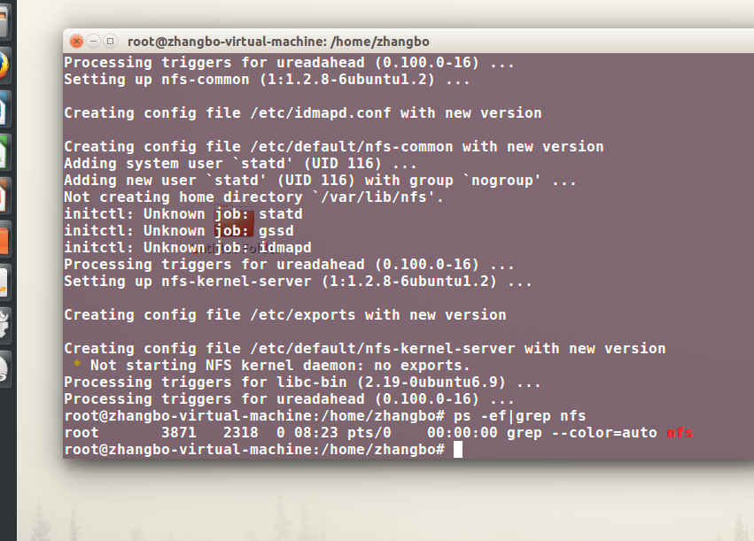
nfs:  1.dpkg -l|grep -i nfs  2.apt-get install nfs-kernel-server 3.启动: service nfs-kernel-server restart

看服务ps -ef

 

 

 

 

 

 

 

 

 

---

2018-08-04,10点03做智能运维.
https://github.com/linjinjin123/awesome-AIOps#white-paper
什么都没有,只能自己找网上题目做

---

不要憎恨你的敌人,那会影响你的判断力 Never hate your enemy, it affects your judgment.教父3

---

 

 

 

 

 

 

 

 

---

 

汇编:

http://study.163.com/course/courseLearn.htm?courseId=1640004#/learn/video?lessonId=1962114&courseId=1640004

win10没法用debug功能:这么解决.

https://blog.csdn.net/lcr_happy/article/details/52491107 

 

 

 指令以16进制存在内存中,本质是2进制.我们看起来是16的.比如FFH 表示255  最后H表示结尾.

数据也一样,都放内存中.

内存中最小单元叫字节bytes=2个16进制数字.也就是8位

cpu的地址线能决定cpu能找到多少个地址. 找到2的N次幂个地址

一个cpu的寻之能力8kb,那么他地址线多宽:2^n=8*1024=2^13所以n=13

一kb存储1024个Byte 一个Byte存储8个bit   就看有没有写e.写e的大,不写e的小.

1KB的存储器有1024个存储单元.

 ROM:只允许读取  电没了还有

RAM:可以写入      电没了就没了

 

 

寄存器里面数字的表示:

AX=AH+AL

BX=BH+BL

CX=CH+CL

DX=DH+DL

16位=8位+8位.所以既可以16位直接mov 也可以移动上8位或者下8位.

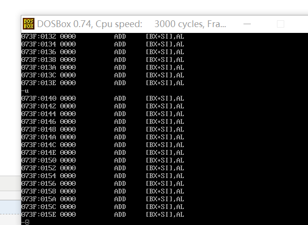
实例:先-r 然后-a 回车 mov ax,4E20回车 再回车 再-t 再-r就发现ax数值变了 (这里面的回车很烦).

 

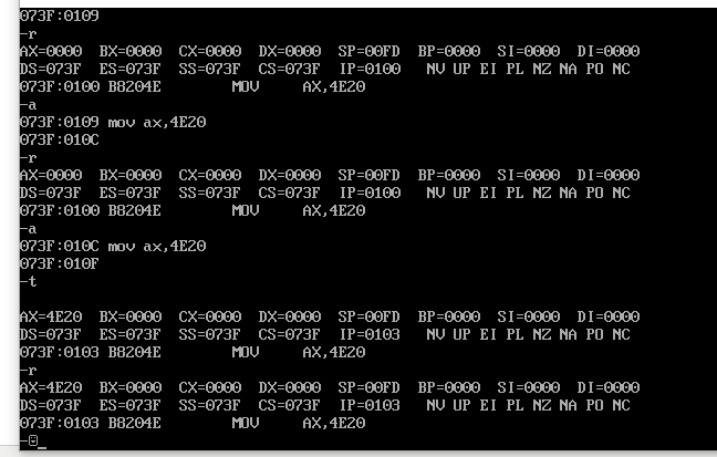
挺乱套的,输入-a之后的命令,他会自己记录下来,不管输入多少,然后每一次-t就按顺序执行一个.

最后发现 mov ah,al 这种也一样能跑.随便位置都能随便mov

 例子:

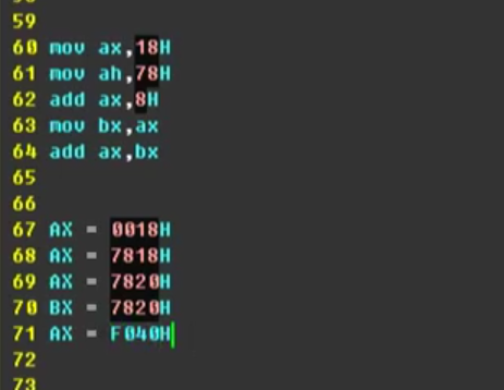
上面5条按顺序跑完就是下面对应5条.H表示的是16进制的数,闲麻烦就直接计算器.选16进制加法

把2个16进制的数7820相加即可.

 

mov ax,8226H

mov bx,ax

add bx,ax 

那么结果是044C 也就是最高位超过了表示范围自动扔掉. (真正敲的时候必须不输入H)

 

物理地址=段地址*16(也就是乘以10H)+偏移地址    

例如:用1230H 和c8表示饿了12300+c8=123c8H这个5个数位的16进制,一个16进制是4byte,所以一共可以表示20byte.

8080cpu就是20byte的地址.用的这种表示方法.

 

 

cup是怎么区分指令和数据的?

cpu把cs:ip 这连个寄存器组成的地址里面的内容当成指令的

 

运行过程:非常重呀!!!!!!!!!!!!!!!!!

  

4个8进制是一个字节,2个16进制也是1个字节

---

 

C premier Plus 书:

1.字是设计计算机时给定的自然的存储单位. 8位机表示一个字是8位,目前64位机表示一个字是64位.而字节是所有计算机都8位.

32位机就是说用32位的数来表示一个整数.也就是正负2^31次幂.

0前缀表示8进制的数,比如020

0x表示16进制的数.

 int cost=12.99   结果是cost=12

float pi=3.1415926   结果是pi是float,只有前6位有精度.

所以定义类型的时候如果不符合会自动强转换成定义的类型,但是精度和数据会变化.

 

 一般而言， 根据%s转换说明， scanf()只会读取字符串中的一个单词， 而不是一整句。 

字符串常量"x"和字符常量'x'不同。 区别之一在于'x'是基本类型
（char） ， 而"x"是派生类型（char数组） ； 区别之二是"x"实际上由两个字符
组成： 'x'和空字符\0（见图4.3） 。

 

 

 

 

 

 

 

---

 

win10 安装redis:

https://blog.csdn.net/thousa_ho/article/details/71279852

按照这个可以进入.

 输入redis-cli.exe

设置键值对 set myKey abc

取出键值对 get myKey

mset a 30 b 20 c 10

mget a b c

 

rpush mylist A

rpush mylist B

lpush mylist first

lrange mylist 0 -1   读取整个列表

 

rpush mylist 1 2 3 4 5 "foo bar"

 

lrange mylist 0 -1

 

rpush mylist 1 2 3 4 5 "foo bar"

rpop mylist

 

hmset user:1000 username antirez birthyear 1977 verified 1   建立一个user:1000哈希表

hget user:1000 username                 读取哈希表

 

hincrby user:1000 birthyear 10       

 

sadd myset 1 2 3

smembers myset

 

 

 

 

 

 

 

 

 

 

 

---

 

 

autohotkey 鼠标连点 的代码:2018-08-11,13点16

$LButton::
Loop
{
  GetKeyState,State,LButton,P
  If (State="U")
  {
    Break
  }
  Else
  {
   
    Send {LButton}
    Sleep 50
  }
}
Return

 

 

 

 

 

---

 

歌曲it is my life

转载于:https://www.cnblogs.com/zhangbo2008/p/9261532.html