


1.1 The Elements of Programming
1.1.1 Expressions
advantage of prefix notation:
1. take an arbitrary number of argument
> (+ 21 34 12 7)
74> (+ (* 3 5) (- 10 6))
191.1.2 Naming and the Environment
we use define to name things:
> (define radius 10)
> (* pi (* radius radius))
314.1592653589793
> (define circumference (* 2 pi radius))
> circumference
62.83185307179586
1.1.3 Evaluating Combinations
evaluating combinations by two steps:
1.1.4 Compound Procedures
powerful elements:
1. Numbers and arithmetic operations are primitive data and procedures.
(define (<name> <formal parameters>) <body>)(define (square x) (* x x))
(define (sum-of-squares x y)
(+ (square x) (square y)))
;25
(sum-of-squares 3 4)1.1.5 The Substitution Model for Procedure Application
The application process is as follows:
To apply a compound procedure to arguments, evaluate the body of the procedure with each formal parameter replaced by the corresponding argument.
so, (sum-of-squares 3 4) first to be:
(sum-of-squares 3 4)
-> (+ (square 3) (square 4))
-> (+ (* 3 3) (* 4 4))
-> (+ 9 16)
-> 25but there has another evaluation: normal-order evaluation.
(define (square x) (* x x))
(define (sum-of-squares x y)
  (+ (square x) (square y)))
(define (f a)
  (sum-of-squares (+ a 1) (* a 2)))

;normal-order evaluation
(sum-of-squares (+ 5 1) (* 5 2))
-> (+ (square (+ 5 1)) (square (* 5 2)))
-> (+ (* (+ 5 1) (+ 5 1)) (* (* 5 2) (* 5 2)))
-> (+ (* 6 6) (* 10 10))
-> (+ 36 100)
-> 136

;applicative-order evaluation
(sum-of-squares (+ 5 1) (* 5 2))
-> (+ (square 6) (square 10))
-> (+ (* 6 6) (* 10 10))
-> (+ 36 100)
-> 1361.1.6 Conditional Expressions and Predicates
conditional expression is:
(cond (<p1> <e1>)
          (<p2> <e2>)
          ...
          (<pn> <en>))
(cond (<p1> <e1>
          (<p2> <e2>)
          ...
          (<pn> <en>)
          (else <e>)))
(if <predicate> <consequent> <alternative>)(define (abs x)
(cond ((> x 0) x)
((= x 0) 0)
((< x 0) (- x))))
;better use else
(define (abs x)
(cond ((< x 0) (- x))
(else
x)))
;also use if
(define (abs x)
(if (< x 0)
(- x)
x))1.1.7 Example:Square Roots by Newton’s Method
how could we accumulate the square-root:
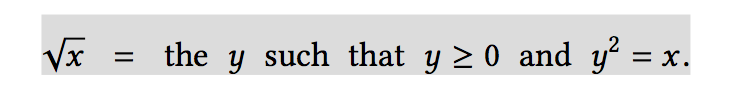
we could use Newton’s method of successive approximations, which says that whenever we have a guess y for the value of the square root of a number x, we can perform a simple manipulation to get a better guess(one closer to the actual square root) by averaging y with x/y. For example:

we could write LISP code:
(define (sqrt-iter guess x)
  (if (good-enough? guess x)
      guess
      (sqrt-iter (improve guess x) x)))

(define (improve guess x)
  (average guess (/ x guess)))

(define (average x y)
  (/ (+ x y) 2))

(define (good-enough? guess x)
  (< (abs (- (square guess) x)) 0.001))

(define (square x) (* x x))

(define (new-sqrt x)
  (sqrt-iter 1.0 x))

;3.00009155413138
(new-sqrt 9)
;11.704699917758145
(new-sqrt 137)
1.1.8 Procedures as Black-Box Abstractions
Local names:
A formal parameter of a procedure has a very special role in the procedure definition, in that it doesn’t matter what name the formal parameter has. Such a name in called a bound variable, and we say that the procedure definition binds its formal parameters. The meaning of a procedure definition is unchanged if a bound variable is consistently renamed throughout the definition. If a variable is not bound, we say that it is free. The set of expressions for which a binding defines a name is called the scope of that name. In a procedure definition, the bound variables declared as the formal parameters of the procedure have the body of the procedure as their scope.
Internal definitions and block structure:
the sqrt function has a problem that: like good-enough?, improve and sqrt-iter function, it only be using for sqrt, not for others. so we could define them in internal:
(define (new-sqrt x)
  (define (square x) (* x x))
  (define (good-enough? guess x)
    (< (abs (- (square guess) x)) 0.001))
  (define (average x y)
    (/ (+ x y) 2))
  (define (improve guess x)
    (average guess (/ x guess)))
  (define (sqrt-iter guess x)
    (if (good-enough? guess x)
        guess
        (sqrt-iter (improve guess x) x)))
  (sqrt-iter 1.0 x))

;3.00009155413138
(new-sqrt 9)
;11.704699917758145
(new-sqrt 137)because the x will not be changed, we also write like that:
(define (new-sqrt x)
  (define (square x) (* x x))
  (define (good-enough? guess)
    (< (abs (- (square guess) x)) 0.001))
  (define (average x y)
    (/ (+ x y) 2))
  (define (improve guess)
    (average guess (/ x guess)))
  (define (sqrt-iter guess)
    (if (good-enough? guess)
        guess
        (sqrt-iter (improve guess))))
  (sqrt-iter 1.0))

;3.00009155413138
(new-sqrt 9)
;11.704699917758145
(new-sqrt 137)
1.2 Procedures and the Processes They Generate
1.2.1 Linear Recursion and Iteration
when we considering the factorial function:
n! = n · (n − 1) · (n − 2) · · · 3 · 2 · 1.
n! = n · [(n − 1) · (n − 2) · · · 3 · 2 · 1] = n · (n − 1)!
(define (factorial n)
  (if (= n 1)
      1
      (* n (factorial (- n 1)))))
;120
(factorial 5)
(define (factorial n)
  (define (iter-factorial product counter)
    (if (> counter n)
        product
        (iter-factorial (* product counter)
                        (+ counter 1))))
  (iter-factorial 1 1))

;120
(factorial 5) 1.2.2 Tree Recursion
we could write the Fibonacci:
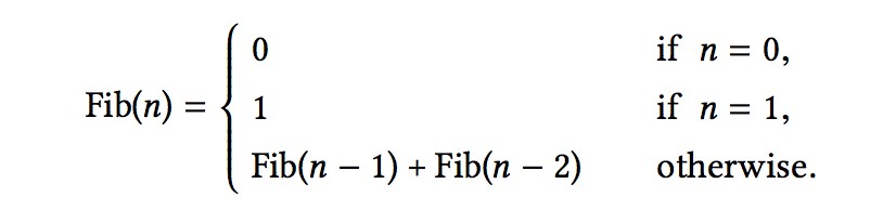
then we write the lisp code:
(define (fib n)
  (cond ((= n 0) 0)
        ((= n 1) 1)
        (else (+ (fib (- n 1))
                 (fib (- n 2))))))
;55
(fib 10)
it’s a tree recursion, like that:

we could also write it in iteration:
(define (fib-recursive n)
  (define (iter-fib a b count)
    (if (= count n)
        a
        (iter-fib b (+ a b) (+ count 1))))
  (iter-fib 0 1 0))

;55
(fib-recursive 10)
Example: Counting change
(define (count-change amount) (cc amount 5))

(define (cc amount kinds-of-coins)
  (cond
    ;amount == 0,1 method
    ((= amount 0) 1)
    ((or (< amount 0) (= kinds-of-coins 0)) 0)
    (else (+
           ;the number of ways to change amount using all but the
           ;first kind of coin(kinds-of-coins - 1)
           (cc amount (- kinds-of-coins 1))
           ;the number of ways to change amount - the value of kinds-of-coins
           (cc (- amount (first-denomination kinds-of-coins)) kinds-of-coins)))))

(define (first-denomination kinds-of-coins)
  (cond ((= kinds-of-coins 1) 1)
        ((= kinds-of-coins 2) 5)
        ((= kinds-of-coins 3) 10)
        ((= kinds-of-coins 4) 25)
        ((= kinds-of-coins 5) 50)))

;292
(count-change 100)
1.2.3 Orders of Growth
the question is: when x is small, sin x == x. so we accumulate the sin x = 3sin(x / 3) - 4sin^3(x / 3):
(define (cube x) (* x x x))

(define (p x) (- (* 3 x) (* 4 (cube x))))

(define (sine angle)
  (if (not (> (abs angle) 0.1))
      angle
      (p (sine (/ angle 3.0)))))

(sine 12.15)
-> (p (sine 405 / 100))
-> (p (p (sine 135 / 100)))
-> (p (p (p (sine 45 / 100))))
-> (p (p (p (p (sine 15 / 100)))))
-> (p (p (p (p (p (sine 5 / 100))))))
-> (p (p (p (p (p 0.05)))))1.2.4 Exponentiation
when we accumulate the b^n, we have two method: the recursive and the iteration:(define (expt-recursive b n)
(if (= n 0)
1
(* b (expt-recursive b (- n 1)))))
(define (expt-iteractive b n)
(define (iter-expt index product)
(if (= index n)
product
(iter-expt (+ index 1) (* product b))))
(iter-expt 1 b))
;1024
(expt-recursive 2 10)
;1024
(expt-iteractive 2 10)(define (square x) (* x x))
(define (fast-expt b n)
(cond ((= n 0) 1)
((even? n) (square (fast-expt b (/ n 2))))
(else
(* b (fast-expt b (- n 1))))))
;1024
(fast-expt 2 10)1.2.5 Greatest Common Divisors
GCD(a, b) = GCD(b, r), r = a % b. so the code like that:
(define (gcd-recursive a b)
  (if (= b 0)
      a
      (gcd-recursive b (remainder a b))))

;4
(gcd-recursive 204 40)
1.2.6 Example: Testing for Primality
Searching for divisors
we could use the stupid method to find the prime:
(define (smallest-divisor n) (find-divisor n 2))

(define (find-divisor n test-divisor)
  (cond ((> (square test-divisor) n) n)
        ((divides? test-divisor n) test-divisor)
        (else
         (find-divisor n (+ test-divisor 1)))))

(define (divides? a b) (= (remainder b a) 0))

(define (square x) (* x x))

(define (prime? n)
  (= n (smallest-divisor n)))

;#t
(prime? 101)
;#f
(prime? 99)(define (square x) (* x x))
(define (expmod base exp m)
(cond ((= exp 0) 1)
((even? exp)
(remainder
(square (expmod base (/ exp 2) m))
m))
(else
(remainder
(* base (expmod base (- exp 1) m))
m))))
(define (fermat-test n)
(define (try-it a)
(= (expmod a n n) a))
(try-it (+ 1 (random (- n 1)))))
(define (fast-prime? n times)
(cond ((= times 0) true)
((fermat-test n) (fast-prime? n (- times 1)))
(else false)))
;#t
(fast-prime? 101 3)
;#f
(fast-prime? 99 3)1.3 Formulating Abstractions with Higher-Order Procedures
1.3.1 Procedures as Arguments
consider the following three procedures:
(define (sum-integers a b)
  (if (> a b)
      0
      (+ a (sum-integers (+ a 1) b))))

(define (sum-cubes a b)
  (if (> a b)
      0
      (+ (cube a)
         (sum-cubes (+ a 1) b))))

(define (pi-sum a b)
  (if (> a b)
      0
      (+ (/ 1.0 (* a (+ a 2)))
(pi-sum (+ a 4) b))))(define (<name> a b)
(if (> a b)
0
(+ (<term> a)
(<name> (<next> a) b)))) 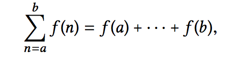
so we now could write our code:
(define (sum term a next b)
  (if (> a b)
      0
      (+ (term a)
         (sum term (next a) next b))))

(define (inc n) (+ n 1))
(define (cube x) (* x x x))
(define (sum-cubes a b)
  (sum cube a inc b))
;3025
(sum-cubes 1 10)

(define (sum-integers a b)
  (sum identity a inc b))
;55
(sum-integers 1 10)

(define (pi-sum a b)
  (define (pi-term x)
    (/ 1.0 (* x (+ x 2))))
  (define (pi-next x)
    (+ x 4))
  (sum pi-term a pi-next b))
;3.141392653591793
(* 8 (pi-sum 1 10000)) 
the code is:
(define (sum term a next b)
  (if (> a b)
      0
      (+ (term a)
         (sum term (next a) next b))))

(define (integral f a b dx)
  (define (add-dx x)
    (+ x dx))
  (* (sum f (+ a (/ dx 2.0)) add-dx b) dx))

(define (cube x) (* x x x))
;0.24998750000000042
(integral cube 0 1 0.01)
;0.249999875000001
(integral cube 0 1 0.001)
1.3.2 Constructing Procedures Using lambda
lambda define that:
(lambda (<formal-paramters>) <body>)(define (plus4 x) (+ x 4))
-> (define plus4 (lambda (x) (+ x 4)))if we accumulate:
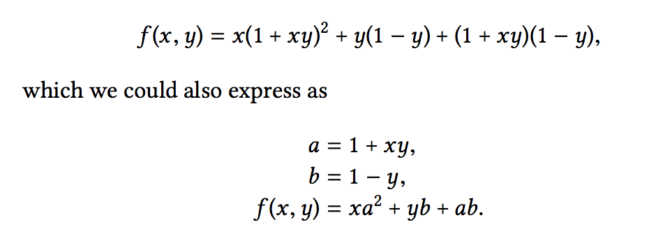
so we first must write like that:
(define (f x y)
  (define (f-helper a b)
    (+ (* x (square a b))
       (* y b)
       (* a b)))
  (f-helper (+ 1 (* x y))
(- 1 y)))(define (f x y)
((lambda (a b)
(+ (* (square a))
(* y b)
(* a b)))
(+ 1 (* x y))
(- 1 y)))(define (f x y)
(let ((a (+ 1 (* x y)))
(b (- 1 y)))
(+ (* x (square a))
(* y b)
(* a b)))) 
and it is a syntactic sugar for the lambda:

there has two way to notice the let:
1. let allows one to bind variables as locally as possible to where they are to be used. For example, if the value of x is 5, the value of the expression:
(+ (let ((x 3))
     (+ x (* x 10)))
x)(let ((x 3)
(y (+ x 2)))
(* x y))1.3.3 Procedures as General Methods
Finding roots of equations by the half-interval methodthe half-interval method use to find roots make f(x) = 0.
(define (average x y) (/ (+ x y) 2.0))
(define (search f neg-point pos-point)
  (let ((midpoint (average neg-point pos-point)))
    (if (close-enough? neg-point pos-point)
        midpoint
        (let ((test-value (f midpoint)))
          (cond ((positive? test-value)
                 (search f neg-point midpoint))
                ((negative? test-value)
                 (search f midpoint pos-point))
                (else midpoint))))))

(define (close-enough? x y) (< (abs (- x y)) 0.01))

(define (half-interval-method f a b)
  (let ((a-value (f a))
        (b-value (f b)))
    (cond ((and (negative? a-value) (positive? b-value))
           (search f a b))
          ((and (negative? b-value) (positive? a-value))
           (search f b a))
          (else
           (error "Values are not of opposite sign" a b)))))
;3.14453125
(half-interval-method sin 2.0 4.0)
(define tolerance 0.00001)
(define (fixed-point f first-guess)
  (define (close-enough? v1 v2)
    (< (abs (- v1 v2))
       tolerance))
  (define (try guess)
    (let ((next (f guess)))
      (if (close-enough? guess next)
          next
          (try next))))
  (try first-guess))
;0.7390822985224023
(fixed-point cos 1.0)
(define (sqrt x)
  (fixed-point (lambda (y) (/ x y))
1.0))(define tolerance 0.00001)
(define (fixed-point f first-guess)
(define (close-enough? v1 v2)
(< (abs (- v1 v2))
tolerance))
(define (try guess)
(let ((next (f guess)))
(if (close-enough? guess next)
next
(try next))))
(try first-guess))
(define (average x y) (/ (+ x y) 2))
(define (sqrt-new x)
(fixed-point (lambda (y) (average y (/ x y)))
1.0))
;3.3166247903554
(sqrt-new 11)1.3.4 Procedures as Returned Values
we use the average to accumulate the y = x ^ 2, we could also use:
(define (average-damp f)
(lambda (x) (average x (f x))))(define (sqrt x)
(fixed-point (average-damp (lambda (y) (/ x y)))
1.0))for the method:

when g(x) = 0, x->f(x). so that is why when g(x) = y^2 - x = 0, we could accumulate sqrt x.
but we first accumulate the Dg(x):

we could write the code:
(define (deriv g)
  (lambda (x) (/ (- (g (+ x dx)) (g x)) dx)))
(define dx 0.00001)
(define (deriv g)
(lambda (x) (/ (- (g (+ x dx)) (g x)) dx)))
(define dx 0.00001)
(define (newton-transform g)
(lambda (x) (- x (/ (g x) ((deriv g) x)))))
(define (newtons-method g guess)
(fixed-point (newton-transform g) guess))
(define (square x) (* x x))
(define (sqrt-new x)
(newtons-method
(lambda (y) (- (square y) x)) 1.0))
(define tolerance 0.00001)
(define (fixed-point f first-guess)
(define (close-enough? v1 v2)
(< (abs (- v1 v2))
tolerance))
(define (try guess)
(let ((next (f guess)))
(if (close-enough? guess next)
next
(try next))))
(try first-guess))
;3.316624790355423
(sqrt-new 11)


 2147
2147

 被折叠的 条评论
为什么被折叠?
被折叠的 条评论
为什么被折叠?
 到【灌水乐园】发言


