


电信公司希望对有流失倾向的客户进行挽留。数据分析人员从公司提前了客户基本信息(出生年月等)、社区信息(社区平均收入等)和6个之内的业务信息(通话时间长等),附件为数据及字段说明。
导入数据和数据清洗
> setwd('C:\\Users\\Xu\\Desktop\\data')
> telecom_churn<-read.csv("telecom_churn.csv")
> telecom_churn<-na.omit(telecom_churn)
> attach(telecom_churn)
随机抽样,建立训练集与测试集
> set.seed(100)
> select<-sample(1:nrow(telecom_churn),nrow(telecom_churn)*0.7)
> train=telecom_churn[select,]  #训练集
> test=telecom_churn[-select,]  #样本集
拟合模型,并且根据逐步回归选择更优的模型,AIC越小模型越优
> lg<-glm(churn~AGE+edu_class+incomeCode+duration+feton+peakMinAv+peakMinDiff,family=binomial(link='logit'))
> summary(lg)

Call:
glm(formula = churn ~ AGE + edu_class + incomeCode + duration +
    feton + peakMinAv + peakMinDiff, family = binomial(link = "logit"))

Deviance Residuals:
     Min        1Q    Median        3Q       Max
-3.07235  -0.58919  -0.03107   0.62704   2.73329

Coefficients:
              Estimate Std. Error z value Pr(>|z|)
(Intercept)  3.3456176  0.2522880  13.261  < 2e-16 ***
AGE         -0.0229400  0.0042145  -5.443 5.24e-08 ***
edu_class    0.4476978  0.0719659   6.221 4.94e-10 ***
incomeCode   0.0071214  0.0033891   2.101   0.0356 *
duration    -0.2641532  0.0126729 -20.844  < 2e-16 ***
feton       -1.0583303  0.1153652  -9.174  < 2e-16 ***
peakMinAv    0.0001973  0.0004272   0.462   0.6441      #并不显著
peakMinDiff -0.0028613  0.0003654  -7.830 4.87e-15 ***
---
Signif. codes:  0 ‘***’ 0.001 ‘**’ 0.01 ‘*’ 0.05 ‘.’ 0.1 ‘ ’ 1

(Dispersion parameter for binomial family taken to be 1)

    Null deviance: 3336.6  on 2423  degrees of freedom
Residual deviance: 1898.2  on 2416  degrees of freedom
AIC: 1914.2

Number of Fisher Scoring iterations: 6

> lg_ms<-step(lg,direction = "both") #寻找最好的回归模型,both向前,向后回归
Start:  AIC=1914.21
churn ~ AGE + edu_class + incomeCode + duration + feton + peakMinAv +
    peakMinDiff

              Df Deviance    AIC
- peakMinAv    1   1898.4 1912.4
<none>             1898.2 1914.2
- incomeCode   1   1902.6 1916.6
- AGE          1   1928.4 1942.4
- edu_class    1   1938.5 1952.5
- peakMinDiff  1   1967.8 1981.8
- feton        1   1985.8 1999.8
- duration     1   2954.6 2968.6

Step:  AIC=1912.43
churn ~ AGE + edu_class + incomeCode + duration + feton + peakMinDiff

              Df Deviance    AIC
<none>             1898.4 1912.4
+ peakMinAv    1   1898.2 1914.2
- incomeCode   1   1902.8 1914.8
- AGE          1   1930.8 1942.8
- edu_class    1   1938.7 1950.7
- peakMinDiff  1   1968.0 1980.0
- feton        1   1986.1 1998.1
- duration     1   2954.8 2966.8
> summary(lg_ms)

Call:
glm(formula = churn ~ AGE + edu_class + incomeCode + duration +
    feton + peakMinDiff, family = binomial(link = "logit"))

Deviance Residuals:
     Min        1Q    Median        3Q       Max
-3.01069  -0.58881  -0.03095   0.62815   2.72788

Coefficients:
              Estimate Std. Error z value Pr(>|z|)
(Intercept)  3.3989882  0.2247215  15.125  < 2e-16 ***
AGE         -0.0233168  0.0041359  -5.638 1.72e-08 ***
edu_class    0.4478730  0.0719857   6.222 4.92e-10 ***
incomeCode   0.0070731  0.0033873   2.088   0.0368 *
duration    -0.2641731  0.0126728 -20.846  < 2e-16 ***
feton       -1.0589440  0.1153516  -9.180  < 2e-16 ***
peakMinDiff -0.0028390  0.0003616  -7.851 4.13e-15 ***
---
Signif. codes:  0 ‘***’ 0.001 ‘**’ 0.01 ‘*’ 0.05 ‘.’ 0.1 ‘ ’ 1

(Dispersion parameter for binomial family taken to be 1)

    Null deviance: 3336.6  on 2423  degrees of freedom
Residual deviance: 1898.4  on 2417  degrees of freedom
AIC: 1912.4   #这个AIC更小,所以这个模型更合适

Number of Fisher Scoring iterations: 6
选择模型后对训练集进行预测
> train$lg_p<-predict(lg_ms, train)  #训练集中进行预测
> summary(train$lg_p)
    Min.  1st Qu.   Median     Mean  3rd Qu.     Max.
-15.8300  -2.6670  -0.1845  -0.9950   1.3380   5.3550
逻辑回归算出来的是将事件发生的概率logit,所以我们把他转化回来,这样更易于我们理解它
> train$p<-1/(1+exp(-1*train$lg_p)) #exp():自然对数e为底指数函数
> summary(train$p)  #概率值的概述
     Min.   1st Qu.    Median      Mean   3rd Qu.      Max.
0.0000001 0.0649300 0.4540000 0.4505000 0.7922000 0.9953000
对预测的模型进行评估
> test$lg_p<-predict(lg_ms, test)我们可以直接利用pROC包,直接绘制ROC曲线和AUC值
> library(pROC)
> modelroc <- roc(test$churn,test$lg_p)   #test$churn为预测的变量1为流失,0为未流失, test%lg_p则为拟合的模型
> plot(modelroc,print.auc=T,auc.ploygon=T,grid=c(0.1,0.2),
+      grid.col=c('green','red'),max.auc.polygon=T,
+      auc.ploygon.col='skyblue',
+      print.thres=T)

Call:
roc.default(response = test$churn, predictor = test$lg_p)

Data: test$lg_p in 597 controls (test$churn 0) < 442 cases (test$churn 1).
Area under the curve: 0.9131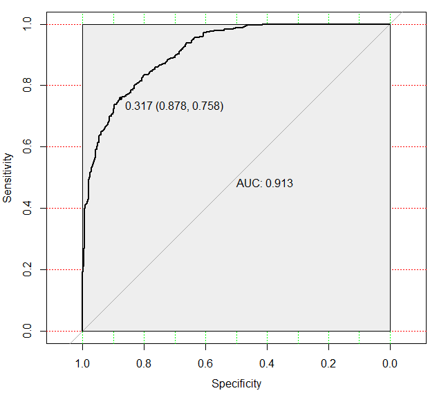
AUC值为0.913,说明模型还是相关可以的
绘制ROC曲线,也可以这样,
> library(ROCR)
There were 50 or more warnings (use warnings() to see the first 50)
> pred_Te <- prediction(test$p, test$churn)
> perf_Te <- performance(pred_Te,"tpr","fpr")
> pred_Tr <- prediction(train$p, train$churn)
> perf_Tr <- performance(pred_Tr,"tpr","fpr")
> plot(perf_Te, col='blue',lty=1);
> plot(perf_Tr, col='black',lty=2,add=TRUE);
> abline(0,1,lty=2,col='red')
> lr_m_auc<-round(as.numeric(performance(pred_Tr,'auc')@y.values),3)
> lr_m_str<-paste("Mode_Train-AUC:",lr_m_auc,sep="")
> legend(0.3,0.4,c(lr_m_str),2:8)
> lr_m_auc<-round(as.numeric(performance(pred_Te,'auc')@y.values),3)
> lr_m_ste<-paste("Mode_Test-AUC:",lr_m_auc,sep="")
> legend(0.3,0.2,c(lr_m_ste),2:8)
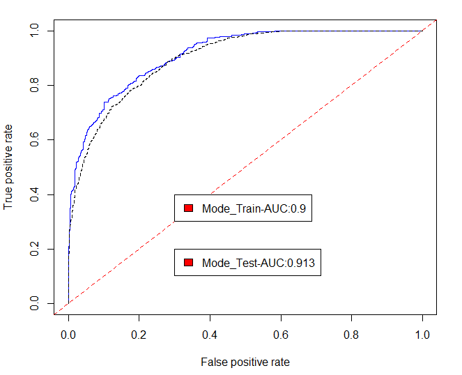
当然这种绘制方法比较麻烦,推荐用第一种那种,这样如果想要进行电信客户流失的预警,就可以用这个模型试试了,算出客户流失的可能性有多大,针对可能流失的客户针对性采取挽留方法。


 2976
2976

 被折叠的 条评论
为什么被折叠?
被折叠的 条评论
为什么被折叠?
 到【灌水乐园】发言


