


本文为《Python深度学习》的学习笔记。
第2章 神经网络的数学基础
2.2.1 标量(0D张量) 2.2.2 向量(1D张量) 2.2.3 矩阵(2D张量) 2.2.4 3D张量和更高维张量
2.2.5 关键属性 2.2.6 在Numpy中操作张量 2.2.7 数据批量的概率 2.2.8 现实世界中的数据张量
2.2.9 向量数据 2.2.10 时间序列数据或序列数据 2.2.11 图像数据 2.2.12 视频数据
2.3.1 逐元素计算(element-wise) 2.3.2 广播 2.3.3 张量点积 2.3.4 张量变形
2.3.5 张量运算的几何解释 2.3.6 深度学习的几何解释
2.4.1 什么是导数 2.4.2 张量运算的导数:梯度 2.4.3 随机梯度下降 2.4.4 链式求导: 反向传播算法
第2章 神经网络的数学基础
2.1 初识神经网络
1.使用MNIST数据集测试神经网络
# 2-1 加载Keras中的MNIST数据集
from keras.datasets import mnist

(train_images, train_labels), (test_images, test_labels) = mnist.load_data()
print(train_images.shape)
print(len(train_labels))
print(train_labels)
print(test_images.shape)
print(len(test_labels))
print(train_labels)
# 输出
(60000, 28, 28)
60000
[5 0 4 ... 5 6 8]
(10000, 28, 28)
10000
[5 0 4 ... 5 6 8]2.神经网络核心组件是层(layer),这是一种数据处理模块,可以看做是一种数据过滤器。下面例子中是由2个Dense层组成,下面是一个10路softmax层,,返回一个由10个概率值组成的数组。
# 2-2 网络架构
from keras import models
from keras import layers

network = models.Sequential()
network.add(layers.Dense(512, activation='relu', input_shape=(28*28,)))
network.add(layers.Dense(10, activation='softmax') )
# 2-3 编译步骤
network.compile(optimizer = 'rmsprop',
loss = 'categorical_crossentropy',
metrics = ['accuracy'])3.准备图像数据及标签
# 2-4 准备图像数据
train_images = train_images.reshape((60000,28 * 28 ))
train_images = train_images.astype('float32') / 255

test_images = test_images.reshape((10000,28 * 28 ))
test_images = test_images.astype('float32') / 255

# 2-5 准备标签
from keras.utils import to_categorical

train_labels = to_categorical(train_labels)
test_labels = to_categorical(test_labels)4.开始训练网络,调用网络拟合模型fit
network.fit(train_images, train_labels, epochs=5, batch_size=128)

# 输出
Epoch 1/5
60000/60000 [==============================] - 8s 137us/step - loss: 0.2556 - acc: 0.9269
Epoch 2/5
60000/60000 [==============================] - 7s 118us/step - loss: 0.1022 - acc: 0.9695
Epoch 3/5
60000/60000 [==============================] - 7s 114us/step - loss: 0.0684 - acc: 0.9801
Epoch 4/5
60000/60000 [==============================] - 7s 113us/step - loss: 0.0498 - acc: 0.9851
Epoch 5/5
60000/60000 [==============================] - 7s 110us/step - loss: 0.0375 - acc: 0.9882
5.测试集精度
test_loss, test_acc = network.evaluate(test_images, test_labels)
print('test_acc',  test_acc)

输出

test_loss, test_acc = network.evaluate(test_images, test_labels)
print('test_acc',  test_acc)
test_loss, test_acc = network.evaluate(test_images, test_labels)
print('test_acc',  test_acc)
10000/10000 [==============================] - 1s 67us/step
test_acc 0.9823
完整代码
from keras.datasets import mnist
from keras import models
from keras import layers
from keras.utils import to_categorical

# 训练数据、测试数据
(train_images, train_labels), (test_images, test_labels) = mnist.load_data()
train_images = train_images.reshape((60000,28 * 28 ))
train_images = train_images.astype('float32') / 255

test_images = test_images.reshape((10000,28 * 28 ))
test_images = test_images.astype('float32') / 255

# 构建网络模型
network = models.Sequential()
network.add(layers.Dense(512, activation='relu', input_shape=(28*28,)))
network.add(layers.Dense(10, activation='softmax') )

# 编译
network.compile(optimizer = 'rmsprop',
                loss = 'categorical_crossentropy',
                metrics = ['accuracy'])

# 准备标签
train_labels = to_categorical(train_labels)
test_labels = to_categorical(test_labels)

# 训练网络并测试
network.fit(train_images, train_labels, epochs=5, batctest_loss, test_acc = network.evaluate(test_images, test_labels)
print('test_acc',  test_acc)h_size=128)
2.2 神经网络的数据表示
张量(tensor)是矩阵的任意维度推广,张量的维度(dimension)通常叫做轴(axis)
2.2.1 标量(0D张量)
仅包含一个数字的张量叫做标量(scalar)。
在numpy中,一个float32或者float64就是一个标量,张量的轴(axis)也叫作阶(rank)
import numpy as np
x = np.array(12)
print(x)
print(x.ndim)

# 输出
12
0
2.2.2 向量(1D张量)
数字组成的数组叫向量(vector)
x = np.array([12, 3, 6, 14, 71])
print(x)
print(x.ndim)

# 输出
[12  3  6 14 71]
1
2.2.3 矩阵(2D张量)
向量组成的数组叫矩阵(matrix)或者二维张量(行和列)。
x = np.array([[5,78,2,34,0],
              [6,79,3,35,1],
              [7,80,4,36,21]])
print(x)
print(x.ndim)

# 输出
[[ 5 78  2 34  0]
 [ 6 79  3 35  1]
 [ 7 80  4 36 21]]
2
2.2.4 3D张量和更高维张量
将多个矩阵组合合成一个新的数组
x = np.array([[[5,78,2,34,0],
              [6,79,3,35,1],
              [7,80,4,36,21]],
              [[5,78,2,34,0],
              [6,79,3,35,1],
              [7,80,4,36,21]],
              [[5,78,2,34,0],
              [6,79,3,35,1],
              [7,80,4,36,21]]])
print(x)
print(x.ndim)

# 输出
[[[ 5 78  2 34  0]
  [ 6 79  3 35  1]
  [ 7 80  4 36 21]]

 [[ 5 78  2 34  0]
  [ 6 79  3 35  1]
  [ 7 80  4 36 21]]

 [[ 5 78  2 34  0]
  [ 6 79  3 35  1]
  [ 7 80  4 36 21]]]
3
2.2.5 关键属性
- 轴的个数ndim
- 形状shape
- 数据类型dtype
from keras.datasets import mnist

(train_images, train_labels), (test_images, test_labels) = mnist.load_data()
print(train_images.ndim)
print(train_images.shape)
print(train_images.dtype)

# 输出
3
(60000, 28, 28)
uint8
使用Matplotlib库来显示这个三维张量中的第四个数字
# 2-6 显示第四个数字
digit = train_images[4]

import matplotlib.pyplot as plt
plt.imshow(digit, cmap=plt.cm.binary)
plt.show()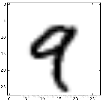
2.2.6 在Numpy中操作张量
- 张量切片train_images[i]
# 下列三种方法等价
my_slice= train_images[10:100]
print(my_slice.shape)
my_slice = train_images[10:100, :, :]
print(my_slice.shape)
my_slice = train_images[10:100, 0:28, 0:28]
print(my_slice.shape)- train_images第一维数据表示第几张图,第二维和第三维表示图片的像素。例如,选取所有图片右下角的14x14像素区域
my_slice = train_images[:, 14:, 14: ]- 也可以使用负数索引,在中心裁剪出14x14像素的区域
my_slice = train_images[:, 7:-7, 7:-7]2.2.7 数据批量的概率
深度学习中所有数据张量的第一个轴都是样本轴,有时也叫作样本维度。通常来说模型每次不会同时处理整个数据集,而是拆分成多个小批量。
batch[0] = train_images[:128]
batch[1] = train_images[128:256]
batch[n] = train_images[128*n:128*(n+1)]
2.2.8 现实世界中的数据张量
- 向量数据:2D张量,形状为(samples, features)
- 时间序列数据或者序列数据:3D张量,形状为(samples, timesteps, features)
- 图像:4D张量,形状为(samples, height, width, channels)或(samples, channels, height, width)
- 视频:5D张量,形状为(samples, frames, height, width, channels)或(samples, frames, channels, height, width)
2.2.9 向量数据
一般为2D张量,第一轴为样本轴,第二维是特征轴
2.2.10 时间序列数据或序列数据
3D张量,特征轴、样本轴、时间步长
2.2.11 图像数据
通常是三个维度:高度、宽度和颜色深度。128张彩色图像组成的批量可以保存在(128, 256, 256, 3)的张量中
2.2.12 视频数据
5D张量,视频每一帧形状为(height, width, color_depth),一系列帧可以保存在形状为(frames, height, width, color_depth),不同视频组成的批量可以保存在一个5D的张量中,形状为(samples, frames, height, width, color_depth)
2.3 神经网络的“齿轮”:张量运算
output = relu(dot(W, input) + b)
拆分来看是dot点积运算、张量与向量b的加法运算、最后的relu运算。
2.3.1 逐元素计算(element-wise)
def naive_relu(x):
    assert len(x.shape) == 2

    x = x.copy()
    for i in range(x.shape[0]):
        for j in range(x.shape[1]):
            x[i,j] = max(x[i, j], 0)
    return x

def naive_add(x):
    assert len(x.shape) == 2
    assert x.shape ==y.shape

    x = x.copy()
    for i in range(x.shape[0]):
        for j in range(x.shape[1]):
            x[i,j] += y[i, j]
    return x
import numpy as np
def elementwise_np(x, y):
z = x + y
z = np.maximum(z, 0.)
return zx = [[1, 1],
[2,2]]
y = [[1, 1],
[2,2]]
z1 = elementwise_np(x, y)
print(z1)2.3.2 广播
naive_add仅支持两个形状相同的2D张量。如果形状不同的张量相加,较小的张量会被广播(broadcast),以匹配较大的张量形状。广播步骤为以下两步:
(1)向较小的张量添加轴,使其ndim与较大的张量相同
(2)将较小的张量沿着新轴重复,使其与较大的张量相同
def naive_add_matrix_and_vector(x, y):
    assert len(x.shape) == 2
    assert len(y.shape) == 1
    assert x.shape[1] == y.shape[0]

    x = x.copy()
    for i in range(x.shape[0]):
        for j in range(x.shape[1]):
            x[i, j] += y[j]
    return x
如果一个张量的形状是(a, b, ... n, n+1, ... m),另一个张量形状是(n, n+1, ... m),那么广播会自动应用于从a到n-1的轴。
# 利用广播将elementwise的maximum运算应用于两个不同的张量
import numpy as np

x = np.random.random((64, 3, 32, 10))
y = np.random.random((32, 10))

z = np.maximum(x, y)
print(z)
2.3.3 张量点积
tensor product,在Numpy、Tensorflow、Theano、Keras中都是用*来实现element-wise。
在Numpy和keras中,用标准的dot运算符实现点积。
import numpy as np
z = np.dot(x, y)
- 数学符号中的点(.)表示点积运算
# 点积运算
def naive_vector_dot(x, y):
    assert len(x.shape) == 1
    assert len(y.shape) == 1
    assert x.shape[0] == y.shape[0]

    z = 0.
    for i in range(x.shape[0]):
        z += x[i] * y[i]
    return z
x = np.array([1, 2])
y = np.array([1, 2])
naive_vector_dot(x,y)
# 输出 5.0 注意这里使用np.array()创建数组,常规的list没有shape这个属性两个向量之间的点积是一个标量,只有元素个数相同的向量(vector)才能做点积
- 同时也可以对一个矩阵x和一个向量y做点积,返回值是一个向量。其中每个元素是y和x每一行之间的点积。
# 矩阵x和一个向量y做点积,返回一个向量
import numpy as np

def naive_matrix_vector_dot(x, y):
    assert len(x.shape) == 2
    assert len(y.shape) == 1
    assert x.shape[1] == y.shape[0]

    z = np.zeros(x.shape[0])
    for i in range(x.shape[0]):
        for j in range(x.shape[1]):
            z[i] += x[i, j] * y[j]
    return z
x = np.array([[1, 1],
[2, 2]])
y = np.array([1, 3])
naive_matrix_vector_dot(x, y)
# 输出 array([4., 8.])两个张量中有一个ndim大于1,那么dot运算就不再对称,则dot(x, y)不等于dot(y, x)
-
点积可以推广到具有任意个轴的张量,两个矩阵间的点积。
对于矩阵x和y,当且仅当x.shape[1] == y.shape[0]时,才能做点积运算dot(x, y),得到的结果为(x.shape[0], y.shape[1])的矩阵。
def naive_matrix_dot(x, y):
    assert len(x.shape) == 2
    assert len(y.shape) == 2
    assert x.shape[1] == y.shape[0]

    z = np.zeros((x.shape[0], y.shape[1]))
    for i in range(x.shape[0]):
        for j in range(y.shape[1]):
            row_x = x[i, :]
            column_y = y[:, j]
            z[i, j] = naive_vector_dot(row_x, column_y)
    return z
# 矩阵x:2x3 矩阵y: 3x2
x = np.array([[1, 1, 1],
[2, 2, 2]])
y = np.array([[1, 1],
[2, 2],
[3, 3]])
naive_matrix_dot(x, y)
# 输出array([[ 6., 6.], [12., 12.]])2.3.4 张量变形
数据预处理时用到train_images = train_images.reshape((60000, 28*28))
x = np.array([[0., 1.],
             [2., 3.],
             [4., 5.]])
print(x.shape)
x = x.reshape((6,1))
print(x)

# 转置transpose
x = np.zeros((300,20))
x = np.transpose(x)
print(x.shape)
# 输出6x1的张量
(3, 2)
[[0.]
[1.]
[2.]
[3.]
[4.]
[5.]]
(20, 300)2.3.5 张量运算的几何解释
二维空间的一个点,向量描绘成原点的箭头。通常来说,仿射变换、旋转、缩放等基本几何操作表示为张量运算。
2.3.6 深度学习的几何解释
将复杂的几何变换逐步分解为一长串基本的几何变换。
2.4 神经网络的“引擎”: 基于梯度的优化
对于网络所有计算都是可微的(differentiable),计算网络系数的梯度,然后反方向改变系数,从而使损失降低
2.4.1 什么是导数
导数(derivative)
2.4.2 张量运算的导数:梯度
梯度是张量运算的导数,输入向量x、一个矩阵W、一个目标y和一个损失函数loss。用W来计算预测值y_pred,然后计算损失(y和y_pred之间的距离)。
y_pred = dot(W, x)
loss_value = loss(y_pred, y)

loss_value = f(W)
W1 = W0 - step * gradient(f)(W0)
2.4.3 随机梯度下降
(1)抽取训练样本x和对于目标y组成的数据批量
(2)在x上运行网络,得到预测值y_pred
(3)计算网络在这批数据上的损失,用于衡量y_pred和y之间的距离
(4)计算损失相对于网络参数的梯度
(5)将参数沿着梯度的反方向移动一点, W -= step * gradient
小批量随机梯度下降(mini-batch stochastic gradient descent)
# 动量方法(momentum)
past_velocity= 0.
momentum= 0.1
while loss > 0.01:
    w, loss, gradient = get_current_parameters()
    velocity = past_velocity * momentum - learning_rate * gradient
    w = w + momentum * velocity - learning_rate * gradient
    past_velocity = velocity
    update_parameter(w)
2.4.4 链式求导: 反向传播算法
backpropagation
2.5 回顾第一个例子
from keras.datasets import mnist
from keras import models
from keras import layers
from keras.utils import to_categorical

# 训练数据、测试数据
(train_images, train_labels), (test_images, test_labels) = mnist.load_data()
train_images = train_images.reshape((60000,28 * 28 ))
train_images = train_images.astype('float32') / 255

test_images = test_images.reshape((10000,28 * 28 ))
test_images = test_images.astype('float32') / 255
# 构建网络模型
network = models.Sequential()
network.add(layers.Dense(512, activation='relu', input_shape=(28*28,)))
network.add(layers.Dense(10, activation='softmax') )
# 编译
network.compile(optimizer = 'rmsprop',
                loss = 'categorical_crossentropy',
                metrics = ['accuracy'])
# 准备标签
train_labels = to_categorical(train_labels)
test_labels = to_categorical(test_labels)# 训练网络并测试
network.fit(train_images, train_labels, epochs=5, batctest_loss, test_acc = network.evaluate(test_images, test_labels)
print('test_acc', test_acc)h_size=128)


 1273
1273


 被折叠的 条评论
为什么被折叠?
被折叠的 条评论
为什么被折叠?
 到【灌水乐园】发言


