


Tensorboard 可视化好助手1
注意: 本节内容会用到浏览器, 而且与 tensorboard 兼容的浏览器是 “Google Chrome”. 使用其他的浏览器不保证所有内容都能正常显示.
学会用 Tensorflow 自带的 tensorboard 去可视化我们所建造出来的神经网络是一个很好的学习理解方式. 用最直观的流程图告诉你你的神经网络是长怎样,有助于你发现编程中间的问题和疑问.
效果
好,我们开始吧。
这次我们会介绍如何可视化神经网络。因为很多时候我们都是做好了一个神经网络,但是没有一个图像可以展示给大家看。这一节会介绍一个TensorFlow的可视化工具 — tensorboard :) 通过使用这个工具我们可以很直观的看到整个神经网络的结构、框架。 以前几节的代码为例:相关代码 通过tensorflow的工具大致可以看到,今天要显示的神经网络差不多是这样子的
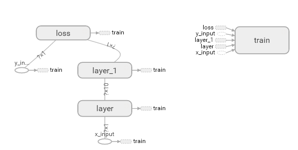
同时我们也可以展开看每个layer中的一些具体的结构:
好,通过阅读代码和之前的图片我们大概知道了此处是有一个输入层(inputs),一个隐含层(layer),还有一个输出层(output) 现在可以看看如何进行可视化.
搭建图纸
首先从 Input 开始:
# define placeholder for inputs to network
xs = tf.placeholder(tf.float32, [None, 1])
ys = tf.placeholder(tf.float32, [None, 1])
对于input我们进行如下修改: 首先,可以为xs指定名称为x_in:
xs= tf.placeholder(tf.float32, [None, 1],name='x_in')然后再次对ys指定名称y_in:
ys= tf.placeholder(tf.loat32, [None, 1],name='y_in')这里指定的名称将来会在可视化的图层inputs中显示出来
使用with tf.name_scope(‘inputs’)可以将xs和ys包含进来,形成一个大的图层,图层的名字就是with tf.name_scope()方法里的参数。
with tf.name_scope('inputs'):
    # define placeholder for inputs to network
    xs = tf.placeholder(tf.float32, [None, 1])
    ys = tf.placeholder(tf.float32, [None, 1])
接下来开始编辑layer , 请看编辑前的程序片段 :
def add_layer(inputs, in_size, out_size, activation_function=None):
    # add one more layer and return the output of this layer
    Weights = tf.Variable(tf.random_normal([in_size, out_size]))
    biases = tf.Variable(tf.zeros([1, out_size]) + 0.1)
    Wx_plus_b = tf.add(tf.matmul(inputs, Weights), biases)
    if activation_function is None:
        outputs = Wx_plus_b
    else:
        outputs = activation_function(Wx_plus_b, )
    return outputs
这里的名字应该叫layer, 下面是编辑后的:
def add_layer(inputs, in_size, out_size, activation_function=None):
    # add one more layer and return the output of this layer
    with tf.name_scope('layer'):
        Weights= tf.Variable(tf.random_normal([in_size, out_size]))
        # and so on...
在定义完大的框架layer之后,同时也需要定义每一个’框架‘里面的小部件:(Weights biases 和 activation function): 现在现对 Weights 定义: 定义的方法同上,可以使用tf.name.scope()方法,同时也可以在Weights中指定名称W。 即为:
 def add_layer(inputs, in_size, out_size, activation_function=None):
    #define layer name
    with tf.name_scope('layer'):
        #define weights name
        with tf.name_scope('weights'):
            Weights= tf.Variable(tf.random_normal([in_size, out_size]),name='W')
        #and so on......
接着继续定义biases , 定义方式同上。
def add_layer(inputs, in_size, out_size, activation_function=None):
    #define layer name
    with tf.name_scope('layer'):
        #define weights name
        with tf.name_scope('weights')
            Weights= tf.Variable(tf.random_normal([in_size, out_size]),name='W')
        # define biase
        with tf.name_scope('Wx_plus_b'):
            Wx_plus_b = tf.add(tf.matmul(inputs, Weights), biases)
        # and so on....
activation_function 的话,可以暂时忽略。因为当你自己选择用 tensorflow 中的激励函数(activation function)的时候,tensorflow会默认添加名称。 最终,layer形式如下:
def add_layer(inputs, in_size, out_size, activation_function=None):
# add one more layer and return the output of this layer
with tf.name_scope('layer'):
with tf.name_scope('weights'):
Weights = tf.Variable(
tf.random_normal([in_size, out_size]),
name='W')
with tf.name_scope('biases'):
biases = tf.Variable(
tf.zeros([1, out_size]) + 0.1,
name='b')
with tf.name_scope('Wx_plus_b'):
Wx_plus_b = tf.add(
tf.matmul(inputs, Weights),
biases)
if activation_function is None:
outputs = Wx_plus_b
else:
outputs = activation_function(Wx_plus_b, )
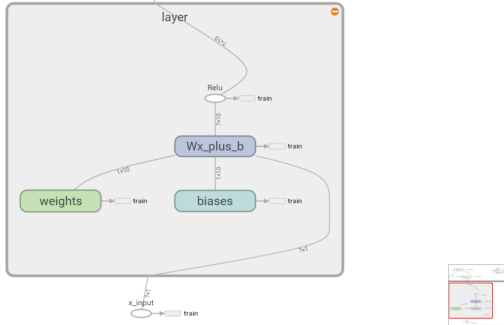
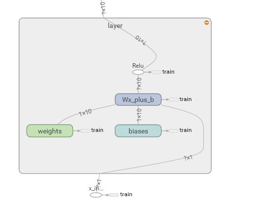
return outputs效果如下:(有没有看见刚才定义layer里面的“内部构件”呢?)
最后编辑loss部分:将with tf.name_scope()添加在loss上方,并为它起名为loss
# the error between prediciton and real data
with tf.name_scope('loss'):
    loss = tf.reduce_mean(
    tf.reduce_sum(
    tf.square(ys - prediction),
    eduction_indices=[1]
    ))
这句话就是“绘制” loss了, 如下:
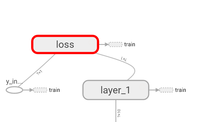
使用with tf.name_scope()再次对train_step部分进行编辑,如下:
with tf.name_scope('train'):
    train_step = tf.train.GradientDescentOptimizer(0.1).minimize(loss)
我们需要使用 tf.summary.FileWriter() (tf.train.SummaryWriter() 这种方式已经在 tf >= 0.12 版本中摒弃) 将上面‘绘画’出的图保存到一个目录中,以方便后期在浏览器中可以浏览。 这个方法中的第二个参数需要使用sess.graph , 因此我们需要把这句话放在获取session的后面。 这里的graph是将前面定义的框架信息收集起来,然后放在logs/目录下面。
sess = tf.Session() # get session
# tf.train.SummaryWriter soon be deprecated, use following
writer = tf.summary.FileWriter("logs/", sess.graph)
最后在你的terminal(终端)中 ,使用以下命令
tensorboard --logdir logs同时将终端中输出的网址复制到浏览器中,便可以看到之前定义的视图框架了。
tensorboard 还有很多其他的参数,希望大家可以多多了解, 可以使用 tensorboard –help 查看tensorboard的详细参数
全部代码:
from __future__ import print_function
import tensorflow as tf


def add_layer(inputs, in_size, out_size, activation_function=None):
    # add one more layer and return the output of this layer
    with tf.name_scope('layer'):
        with tf.name_scope('weights'):
            Weights = tf.Variable(tf.random_normal([in_size, out_size]), name='W')
        with tf.name_scope('biases'):
            biases = tf.Variable(tf.zeros([1, out_size]) + 0.1, name='b')
        with tf.name_scope('Wx_plus_b'):
            Wx_plus_b = tf.add(tf.matmul(inputs, Weights), biases)
        if activation_function is None:
            outputs = Wx_plus_b
        else:
            outputs = activation_function(Wx_plus_b, )
        return outputs


# define placeholder for inputs to network
with tf.name_scope('inputs'):
    xs = tf.placeholder(tf.float32, [None, 1], name='x_input')
    ys = tf.placeholder(tf.float32, [None, 1], name='y_input')

# add hidden layer
l1 = add_layer(xs, 1, 10, activation_function=tf.nn.relu)
# add output layer
prediction = add_layer(l1, 10, 1, activation_function=None)

# the error between prediciton and real data
with tf.name_scope('loss'):
    loss = tf.reduce_mean(tf.reduce_sum(tf.square(ys - prediction),
                                        reduction_indices=[1]))

with tf.name_scope('train'):
    train_step = tf.train.GradientDescentOptimizer(0.1).minimize(loss)

sess = tf.Session()

# tf.train.SummaryWriter soon be deprecated, use following
if int((tf.__version__).split('.')[1]) < 12 and int((tf.__version__).split('.')[0]) < 1:  # tensorflow version < 0.12
    writer = tf.train.SummaryWriter('logs/', sess.graph)
else: # tensorflow version >= 0.12
    writer = tf.summary.FileWriter("logs/", sess.graph)

# tf.initialize_all_variables() no long valid from
# 2017-03-02 if using tensorflow >= 0.12
if int((tf.__version__).split('.')[1]) < 12 and int((tf.__version__).split('.')[0]) < 1:
    init = tf.initialize_all_variables()
else:
    init = tf.global_variables_initializer()
sess.run(init)

# direct to the local dir and run this in terminal:
# $ tensorboard --logdir=logs
可能会遇到的问题
(1) 而且与 tensorboard 兼容的浏览器是 “Google Chrome”. 使用其他的浏览器不保证所有内容都能正常显示.
(2) 同时注意, 如果使用 http://0.0.0.0:6006 网址打不开的朋友们, 请使用 http://localhost:6006, 大多数朋友都是这个问题.
(3) 请确保你的 tensorboard 指令是在你的 logs 文件根目录执行的. 如果在其他目录下, 比如 Desktop 等, 可能不会成功看到图. 比如在下面这个目录, 你要 cd 到 project 这个地方执行 /project > tensorboard –logdir logs
- project
   - logs
   model.py
   env.py
(4) 讨论区的朋友使用 anaconda 下的 python3.5 的虚拟环境, 如果你输入 tensorboard 的指令, 出现报错: “tensorboard” is not recognized as an internal or external command…
解决方法的关键就是需要激活TensorFlow. 管理员模式打开 Anaconda Prompt, 输入 activate tensorflow, 接着按照上面的流程执行 tensorboard 指令.
Tensorboard可视化好帮手2
注意: 本节内容会用到浏览器, 而且与 tensorboard 兼容的浏览器是 “Google Chrome”. 使用其他的浏览器不保证所有内容都能正常显示.
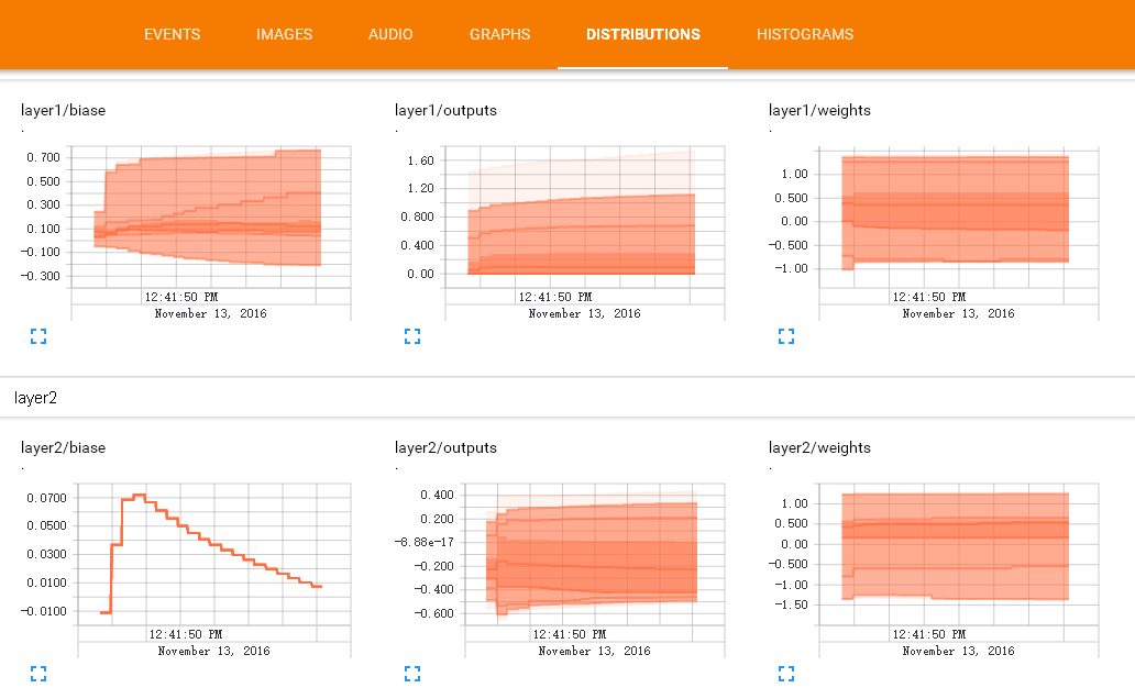
上一篇讲到了 如何可视化TesorBorad整个神经网络结构的过程。 其实tensorboard还可以可视化训练过程( biase变化过程) , 这节重点讲一下可视化训练过程的图标是如何做的 。请看下图, 这是如何做到的呢?
在histograms里面我们还可以看到更多的layers的变化:
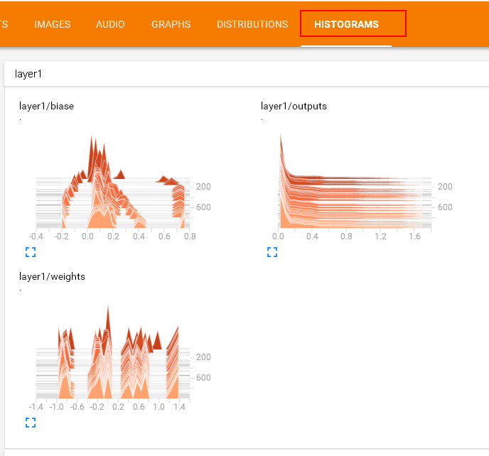
(P.S. 灰猫使用的 tensorflow v1.1 显示的效果可能和视频中的不太一样, 但是 tensorboard 的使用方法的是一样的。)
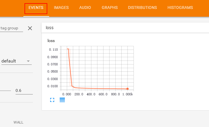
这里还有一个events , 在这次练习中我们会把 整个训练过程中的误差值(loss)在event里面显示出来, 甚至你可以显示更多你想要显示的东西.
好了, 开始练习吧, 本节内容包括:
制作输入源
由于这节我们观察训练过程中神经网络的变化, 所以首先要添一些模拟数据. Python 的 numpy 工具包可以帮助我们制造一些模拟数据. 所以我们先导入这个工具包:
import tensorflow as tf
import numpy as np
然后借助 np 中的 np.linespace() 产生随机的数字, 同时为了模拟更加真实我们会添加一些噪声, 这些噪声是通过 np.random.normal() 随机产生的.
 ## make up some data
 x_data= np.linspace(-1, 1, 300, dtype=np.float32)[:,np.newaxis]
 noise=  np.random.normal(0, 0.05, x_data.shape).astype(np.float32)
 y_data= np.square(x_data) -0.5+ noise
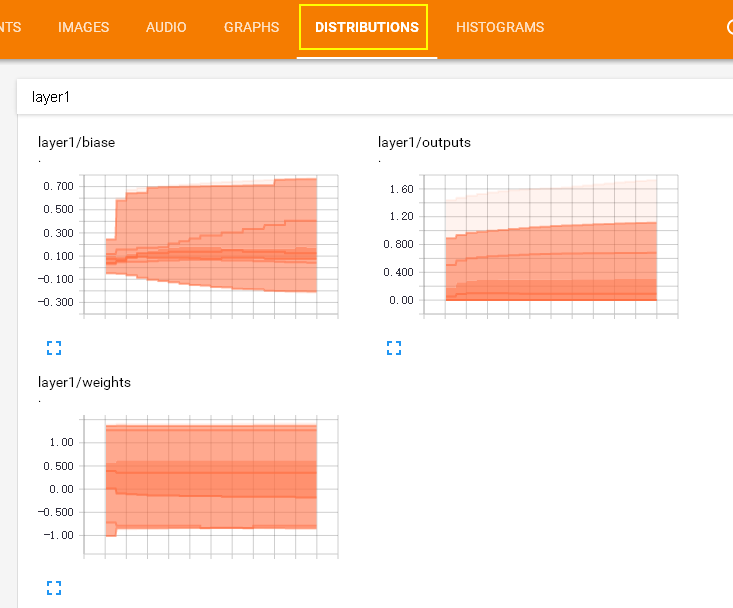
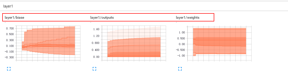
输入源的问题解决之后, 我们开始制作对Weights和biases的变化图表吧. 我们期望可以做到如下的效果, 那么首先从 layer1/weight 做起吧
这个效果是如何做到的呢,请看下一个标题
在 layer 中为 Weights, biases 设置变化图表
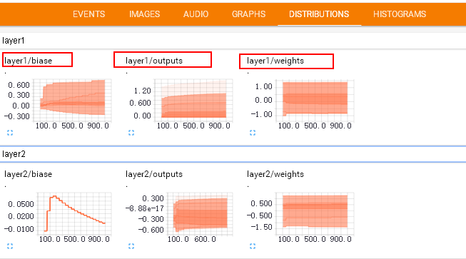
通过上图的观察我们发现每个 layer 后面有有一个数字: layer1 和layer2
于是我们在 add_layer() 方法中添加一个参数 n_layer,用来标识层数, 并且用变量 layer_name 代表其每层的名名称, 代码如下:
def add_layer(
    inputs ,
    in_size,
    out_size,
    n_layer,
    activation_function=None):
    ## add one more layer and return the output of this layer
    layer_name='layer%s'%n_layer  ## define a new var
    ## and so on ……
接下来,我们层中的Weights设置变化图, tensorflow中提供了tf.histogram_summary()方法,用来绘制图片, 第一个参数是图表的名称, 第二个参数是图表要记录的变量
def add_layer(inputs ,
            in_size,
            out_size,n_layer,
            activation_function=None):
    ## add one more layer and return the output of this layer
    layer_name='layer%s'%n_layer
    with tf.name_scope('layer'):
         with tf.name_scope('weights'):
              Weights= tf.Variable(tf.random_normal([in_size, out_size]),name='W')
              # tf.histogram_summary(layer_name+'/weights',Weights)   # tensorflow 0.12 以下版的
              tf.summary.histogram(layer_name + '/weights', Weights) # tensorflow >= 0.12
    ##and so no ……
同样的方法我们对biases进行绘制图标:
with tf.name_scope('biases'):
    biases = tf.Variable(tf.zeros([1,out_size])+0.1, name='b')
    # tf.histogram_summary(layer_name+'/biase',biases)   # tensorflow 0.12 以下版的
    tf.summary.histogram(layer_name + '/biases', biases)  # Tensorflow >= 0.12
至于activation_function 可以不绘制. 我们对output 使用同样的方法:
# tf.histogram_summary(layer_name+'/outputs',outputs) # tensorflow 0.12 以下版本
tf.summary.histogram(layer_name + '/outputs', outputs) # Tensorflow >= 0.12
最终经过我们的修改 , addlayer()方法成为如下的样子:
def add_layer(inputs ,
              in_size,
              out_size,n_layer,
              activation_function=None):
    ## add one more layer and return the output of this layer
    layer_name='layer%s'%n_layer
    with tf.name_scope(layer_name):
         with tf.name_scope('weights'):
              Weights= tf.Variable(tf.random_normal([in_size, out_size]),name='W')
              # tf.histogram_summary(layer_name+'/weights',Weights)
              tf.summary.histogram(layer_name + '/weights', Weights) # tensorflow >= 0.12

         with tf.name_scope('biases'):
              biases = tf.Variable(tf.zeros([1,out_size])+0.1, name='b')
              # tf.histogram_summary(layer_name+'/biase',biases)
              tf.summary.histogram(layer_name + '/biases', biases)  # Tensorflow >= 0.12

         with tf.name_scope('Wx_plus_b'):
              Wx_plus_b = tf.add(tf.matmul(inputs,Weights), biases)

         if activation_function is None:
            outputs=Wx_plus_b
         else:
            outputs= activation_function(Wx_plus_b)

         # tf.histogram_summary(layer_name+'/outputs',outputs)
         tf.summary.histogram(layer_name + '/outputs', outputs) # Tensorflow >= 0.12

    return outputs
修改之后的名称会显示在每个tensorboard中每个图表的上方显示, 如下图所示:
由于我们对addlayer 添加了一个参数, 所以修改之前调用addlayer()函数的地方. 对此处进行修改:
# add hidden layer
l1= add_layer(xs, 1, 10 ,  activation_function=tf.nn.relu)
# add output  layer
prediction= add_layer(l1, 10, 1,  activation_function=None)
添加n_layer参数后, 修改成为 :
# add hidden layer
l1= add_layer(xs, 1, 10, n_layer=1, activation_function=tf.nn.relu)
# add output  layer
prediction= add_layer(l1, 10, 1, n_layer=2, activation_function=None)
设置loss的变化图
Loss 的变化图和之前设置的方法略有不同. loss是在tesnorBorad 的event下面的, 这是由于我们使用的是tf.scalar_summary() 方法.
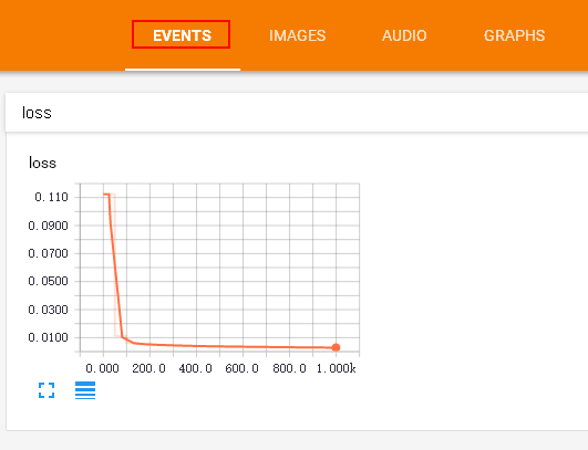
观看loss的变化比较重要. 当你的loss呈下降的趋势,说明你的神经网络训练是有效果的.
修改后的代码片段如下:
with tf.name_scope('loss'):
     loss= tf.reduce_mean(tf.reduce_sum(
              tf.square(ys- prediction), reduction_indices=[1]))
     # tf.scalar_summary('loss',loss) # tensorflow < 0.12
     tf.summary.scalar('loss', loss) # tensorflow >= 0.12
给所有训练图合并
接下来, 开始合并打包。 tf.merge_all_summaries() 方法会对我们所有的 summaries 合并到一起. 因此在原有代码片段中添加:
sess= tf.Session()

# merged= tf.merge_all_summaries()    # tensorflow < 0.12
merged = tf.summary.merge_all() # tensorflow >= 0.12

# writer = tf.train.SummaryWriter('logs/', sess.graph)    # tensorflow < 0.12
writer = tf.summary.FileWriter("logs/", sess.graph) # tensorflow >=0.12

# sess.run(tf.initialize_all_variables()) # tf.initialize_all_variables() # tf 马上就要废弃这种写法
sess.run(tf.global_variables_initializer())  # 替换成这样就好
训练数据
假定给出了x_data,y_data并且训练1000次.
for i in range(1000):
   sess.run(train_step, feed_dict={xs:x_data, ys:y_data})
以上这些仅仅可以记录很绘制出训练的图表, 但是不会记录训练的数据。 为了较为直观显示训练过程中每个参数的变化,我们每隔上50次就记录一次结果 , 同时我们也应注意, merged 也是需要run 才能发挥作用的,所以在for循环中写下:
if i%50 == 0:
    rs = sess.run(merged,feed_dict={xs:x_data,ys:y_data})
    writer.add_summary(rs, i)
最后修改后的片段如下:
for i in range(1000):
   sess.run(train_step, feed_dict={xs:x_data, ys:y_data})
   if i%50 == 0:
      rs = sess.run(merged,feed_dict={xs:x_data,ys:y_data})
      writer.add_summary(rs, i)
在 tensorboard 中查看效果
程序运行完毕之后, 会产生logs目录 , 使用命令 tensorboard –logdir logs
注意: 本节内容会用到浏览器, 而且与 tensorboard 兼容的浏览器是 “Google Chrome”. 使用其他的浏览器不保证所有内容都能正常显示.
同时注意, 如果使用 http://0.0.0.0:6006 或者 tensorboard 中显示的网址打不开的朋友们, 请使用 http://localhost:6006, 大多数朋友都是这个问题.
会有如下输出:
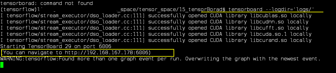
将输出中显示的URL地址粘贴到浏览器中便可以查看. 最终的效果如下:


 2299
2299


 被折叠的 条评论
为什么被折叠?
被折叠的 条评论
为什么被折叠?
 到【灌水乐园】发言


