xpath 统计有几个img标签_成都市租房数据统计分析

成都作为新一线城市，吸引了大量的外来人员，据统计，2019年末成都市常住人口为1658.1万人，比2018年末净增加25.1万人，大量的人员流入带动了成都租房市场的发展。

本文以租房网站上的成都市的租房数据作为参考，针对成都市各区域房源位置，房源数量、租金情况和房源户型等问题，分析成都市租房市场情况。

1. 获取租房数据

获取租房数据的方式有很多，这里我们采用网络爬虫的方式，对链家网上成都市租房数据进行采集。

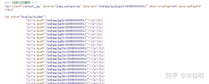
首先打卡链家租房的网址：https://cd.lianjia.com/zufang/rt200600000001/，在页面打开开发者模式，切换到Network。

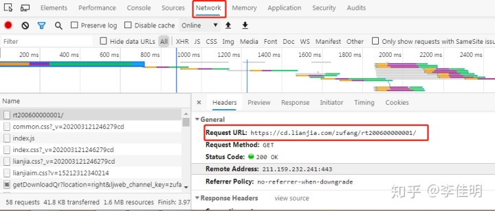
可以很容易的发现Network第一条中对于的URL地址，就是我们所需要爬取的起始地址。

再切换到Elements栏，使用左上角的鼠标选择工具，对网页中的元素进行观察。

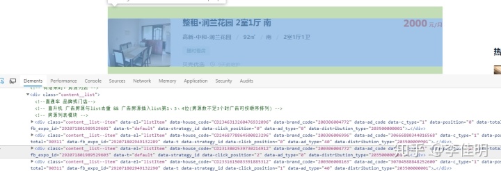
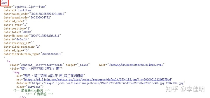
可以发现，每条租房数据都是在一个div标签下。同时我们查看网页源码发现，此处和源码中的情况一致。

再观察网页的翻页情况，可以看到这里通过点击下一页的链接进行翻页。

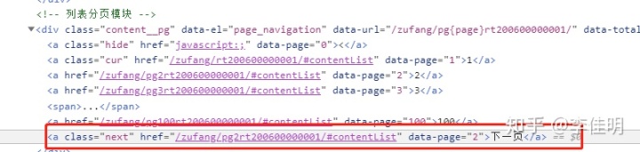
继续查看网页源代码发现，源码里面没有“下一页”相关的内容，取而代之是每页的url地址。

继续查看后面的页面，发现也是这种情况。

由此可见，链家租房每个页面的url地址都在源码中，而且url地址规律十分明显，在此我们可以采用scrapy crawlspider进行快速爬取。

对于规律明显的url地址，scrapy crawlspider可以在编写的规则下自动识别，大大简化了爬虫的编写。

部分代码如下：

import scrapy
from scrapy.linkextractors import LinkExtractor
from scrapy.spiders import CrawlSpider, Rule


class ChuzuSpider(CrawlSpider):
    name = 'zhufang'
    allowed_domains = ['lianjia.com']
    start_urls = ['https://cd.lianjia.com/zufang/rt200600000001/']
    
    # 此处设置查找规则
    rules = (
        Rule(LinkExtractor(allow=r'/zufang/pgd*rt200600000001/'), callback='parse_item', follow=True),
    )

    def parse_item(self, response):
        div_list = response.xpath('//div[@class="content__list"]/div')
        for div in div_list:
            item = {}
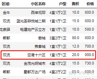
            item['区域:'] = div.xpath('.//p[@class="content__list--item--des"]/a[1]/text()').extract_first()
            item['小区名称'] = div.xpath('.//p[@class="content__list--item--des"]/a[3]/text()').extract_first()
            item['户型'] = div.xpath('.//p[@class="content__list--item--des"]/text()[7]').extract_first().strip()
            item['面积'] = div.xpath('.//p[@class="content__list--item--des"]/text()[5]').extract_first().strip()
            item['价格'] = div.xpath('.//span[@class="content__list--item-price"]/em/text()').extract_first()
            yield item

当然也可以通过其他方式来爬取，这里就不细说了。

最终我们获得了11220条数据。

2. 数据读取与预处理

import pandas as pd
import numpy as np
import matplotlib.pyplot as plt
import matplotlib
%matplotlib inline
# 读取数据
file_path = open(r'C:UsersAdministratorDesktopcodelianjialianjia.csv')
file_data = pd.read_csv(file_path)
file_data.info()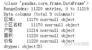

这里列举出了数据集拥有的各类字段，一共有11220个，其中区域、小区名称和户型都存在为空的情况，所有的值均为字符串。

# 查看前五行的数据
file_data.head()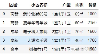

# 处理重复值和空值
# 删除缺失数据，并对file_data重新赋值
file_data = file_data.drop_duplicates()
file_data = file_data.dropna()
file_data.info()

可以看到info中的字段减少了，说明部分重复值和缺失值已经被处理了。

另外，对于面积和价格一栏，我们需要对数据进行进一步的清洗，使其从字符型转换为浮点型，方便后续计算。

# 清洗数据
def clean_data(data):
    position = data.find('㎡')
    data = data[:position]
    return data
data_new = file_data['面积'].apply(clean_data)
data_new.head()

# 转换面积栏数据类型
new_data['面积']= new_data['面积'].astype('float')
new_data.info()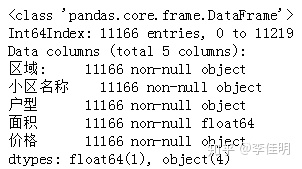

可以看到面积一栏的数据成功转换成了float型。

对于价格一栏，原数据中部分数据存在区间，需要进行处理。

# 处理价格栏的数据
# 定义一个函数处理
def clean_price(data,method):
    position = data.find('-')
    length = len(data)
    if position != -1:  # 判断是否存在区间价格
        bottomPrice = data[:position]
        topPrice = data[position+1:length]
    else:
        bottomPrice = data[:]
        topPrice= bottomPrice
    if method == 'top':
        return topPrice
    else:
        return bottomPrice

函数定义好之后，我们开始对数据进行处理。

new_data['top'] = new_data['价格'].apply(clean_price,method='top')
new_data['bottom'] = new_data['价格'].apply(clean_price,method='bottom')
new_data.top=new_data.top.astype('int')
new_data.bottom=new_data.bottom.astype('int')
#求区间价格平均值
new_data['价格']=new_data.apply(lambda x:(x.top+x.bottom)/2,axis=1)
new_data.drop(['top','bottom'])

再次查看数据，发现区间价格已经被修改。

到此，数据预处理完成。

3.数据分析

3.1 房源位置分析

data_clean.rename(columns={'区域:':'region','小区名称':'community','户型':'houseType','面积':'area','价格':'price'},inplace=True)
data_clean.head()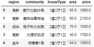

# 统计每个区域房源数量
data_clean.region.value_counts()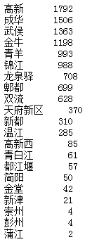

通过结果看出，房源数量前三的为高新区、成华区和武侯区。

接下来我们通过热力图的形式，来展示各区域房源数量的具体分布。获取热力图有多种方法，这里利用百度地图提供的api接口，生成此次所需的热力图。

首先我们需要补全各房源地址。

# 补全地址
data_clean['region'] = data_clean.region.replace('天府新区','天府新')
data_clean['position'] = '成都市'+data_clean.region+'区'+data_clean.community
data_clean.head()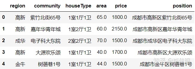

接下来通过房源地址获取经纬度。

# 获取经纬度，生成txt文件
# 需要调用百度地图api
# coding=utf-8
import requests
import pandas as pd
import time
import json
class LngLat:
    # 获取位置一列的数据
    def get_data(self):
        house_names = data_clean['position']
        house_names = house_names.tolist()
        return house_names
    def get_url(self):
        # 替换为自己的ak值
        url_temp = "http://api.map.baidu.com/geocoding/v3/?address={}&output=json&ak=ak值=showLocation"
        house_names = self.get_data()
        return [url_temp.format(i) for i in house_names]
    # 发送请求
    def parse_url(self, url):
        while 1:
            try:
                r = requests.get(url)
            except requests.exceptions.ConnectionError:
                time.sleep(2)
                continue
            return r.content.decode('UTF-8')
    def run(self):
        li = []
        urls = self.get_url()
        for url in urls:
            data = self.parse_url(url)
            str = data.split("{")[-1].split("}")[0]
            try:
                lng = float(str.split(",")[0].split(":")[1])
                lat = float(str.split(",")[1].split(":")[1])
            except ValueError:
                continue
            # 构建字典
            dict_data = dict(lng=lng, lat=lat, count=1)
            li.append(dict_data)
        with open('经纬度信息.txt','w',encoding='UTF-8') as f:
            f.write(json.dumps(li))
        print('正在写入...')
        print('写入成功')
if __name__ == '__main__':    
    execute = LngLat()
    execute.run()

然后根据百度官方的热力图demo进行修改，得到我们所需的热力图。

# 此处仅展示部分代码，详细可见百度地图开发者平台
# 下面为读取上步生成的txt文件
<body>
    <div id="container"></div>
    <div id="r-result">
        上传文件 ： <input type="file" name="file" multiple id="fileId" />
        <button type="submit" name="btn" value="提交" id="btn1" onclick="check()">提交</button>
        <input type="button" onclick="openHeatmap();" value="显示热力图" /><input type="button" onclick="closeHeatmap();"
            value="关闭热力图" />
    </div>
</body>
</html>
<script type="text/javascript">
    var points = [];
    function check() {
        var objFile = document.getElementById("fileId");
        if (objFile.value == "") {
            alert("不能空")
        }
        var files = $('#fileId').prop('files'); //获取到文件列表
        console.log(files.length);
        if (files.length == 0) {
            alert('请选择文件');
        } else {
            for (var i = 0; f = files[i]; i++) {
                var reader = new FileReader(); //新建一个FileReader
                reader.readAsText(files[i], "UTF-8"); //读取文件
                reader.onload = function (evt) { //读取完文件之后会回来这里
                    points = jQuery.parseJSON(evt.target.result);
                }
            }
        } 
    }

在热力图中，颜色越接近红色代表房源数量越多，颜色越接近蓝色代表房源数量越少。从上图看出，大量房源仍集中于传统的五城区之间，另外随着城市的发展，三圣乡、犀浦、高新等区域，也存在着大量的房源。

3.2 户型分析

接下来我们分析一下户型，统计租房市场哪种户型的房源数量偏多。

# 户型数量分析
# 定义函数，用于计算各户型的数量
def all_house(arr):
    arr = np.array(arr)
    key = np.unique(arr)
    result = {}
    for k in key:
        mask = (arr == k)
        arr_new = arr[mask]
        v = arr_new.size
        result[k] = v
    return result
# 获取户型数据
house_array = data_clean['houseType']
house_info = all_house(house_array)
house_type = dict((key, value) for key, value 
in house_info.items() if value > 50) #筛选数量大于50的户型
show_houses = pd.DataFrame({'houseType':[x for x in  house_type.keys()],
                  'count':[x for x in house_type.values()]})
show_houses

为直观的展示结果，可采用条形图进行展示。

matplotlib.rcParams['font.sans-serif'] = ['SimHei']
matplotlib.rcParams['axes.unicode_minus'] = False
house_type = show_houses['houseType']
house_type_num = show_houses['count']
plt.barh(range(17), house_type_num, height=0.7, 
color='steelblue', alpha=0.8)    
plt.yticks(range(17), house_type)
plt.xlim(0,2500)
plt.xlabel("数量")
plt.ylabel("户型种类")
plt.title("成都各户型房屋数量")
for x, y in enumerate(house_type_num):
    plt.text(y + 0.2, x - 0.1, '%s' % y)
plt.show()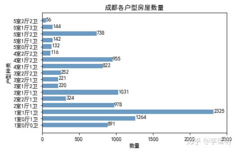

通过上图可以看出，整个租房市场户型数量较多的为小户型的房源，尤其是1室1厅1卫的户型，在整个租房市场数量最多。

3.2 租金分析

针对房租，先用describe函数查看下统计值。

data_clean.price.describe()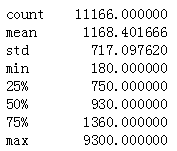

房租的均值为1168，中位数是930，最大房租在9300。标准差为717，有一定的波动性。

# 通过直方图查看房租分布
data_clean.price.hist(bins=20)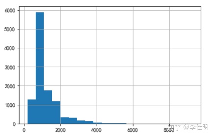

可以看出，绝大部分房租价格位于2000以下。

# 各区域房租价格情况
data_clean.boxplot(column ='price',by='region',figsize=(12,6))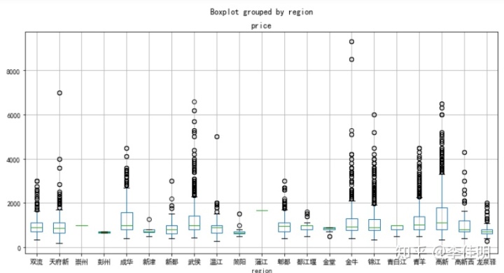

从图上看出，武侯区、成华区、锦江区、金牛区、青羊区、高新区、天府新区、双流区、郫都去等区域的中位数比较接近，而周边区域如简阳、龙泉驿、高新西等，中位数明显等于上述地方。崇州、彭州和蒲江由于样本较少，存在较大的偶然性，暂不考虑。

# 各区域平均租房价格

#求各区域总面积和总金额，及平均价格
avg_price = pd.DataFrame(columns=['sum_price','sum_area','avg_price'])
avg_price['sum_price'] = data_clean.price.groupby(data_clean.region).sum()
avg_price['sum_area'] = data_clean.area.groupby(data_clean.region).sum()
avg_price['avg_price'] = round(avg_price['sum_price']/avg_price['sum_area'],2)
# 合并数据
count = data_clean.groupby(by='region').count()
count.rename(columns={'community':'count'},inplace = True)
avg_price['count'] = count['count']
avg_price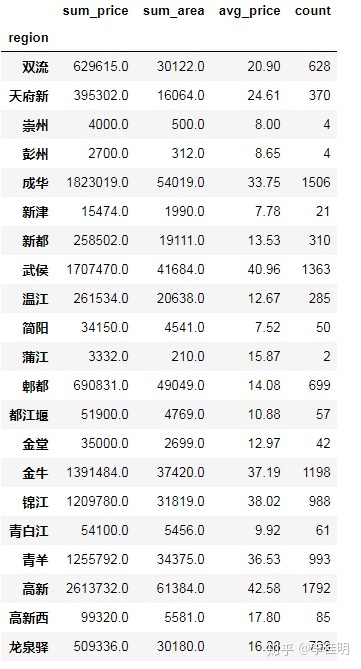

这样，可以将上述数据通过图表来展示。

#图表展示
import matplotlib.ticker as mtick
from matplotlib.font_manager import FontProperties
num= avg_price['count']                 # 数量
price=avg_price['avg_price'] # 价格
l=[i for i in range(21)]
plt.rcParams['font.sans-serif']=['SimHei'] # 设置中文显示
lx=avg_price.index
fig = plt.figure()
fig,ax1=plt.subplots(1,1,figsize=(14,6))
ax1.plot(l, price,'or-',label='价格')
for i,(_x,_y) in enumerate(zip(l,price)):
    plt.text(_x,_y,price[i],color='black',fontsize=10)  
ax1.set_ylim([0, 200])
ax1.set_ylabel('价格（元/平方米）')
plt.legend(prop={'family':'SimHei','size':8},loc='upper left') 
ax2 = ax1.twinx()
plt.bar(l,num,alpha=0.3,color='green',label='数量')
ax2.set_ylabel('数量')
ax2.set_ylim([0, 2000])  
plt.legend(prop={'family':'SimHei','size':8},loc="upper right")
plt.xticks(l,lx)
plt.show()

从上图可以看出，成华区、武侯区、金牛区、锦江区、青羊区和高新区的房源平均价格远大于其他区域的价格，并且高新区的平均价格最高；从房源数量来看，高新区、成华区、武侯区的房源数量为前三，且高新区的房源数量最多。

上述结果主要是因为高新区是成都市最具活力的区域之一，区域内人口众多，经济发达；成华区和武侯区作为传统的主城区，有大量人口居住，相应的房源和价格也会相对提高。

3.3 房源面积分析

针对面积，先用describe函数查看下统计值。

data_clean.price.describe()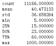

面积的均值为40.47，中位数是23，最大面积为1000，标准差为36。

下面将房源面积按照一定规则划分为多个区间，便于分析哪种面积的房屋更好出租。

首先我们将房屋面积划分为8个区间。

# 面积划分
area_divide = [1, 30, 50, 70, 90, 120, 1200]
area_cut = pd.cut(list(data_clean['area']), area_divide)
area_cut_data = area_cut.describe()
area_cut_data

接着我们通过饼图展示各区间的分布情况。

area_percentage = (area_cut_data['freqs'].values)*100
# 保留两位小数
np.set_printoptions(precision=2)
labels  = ['30平米以下', '30-50平米', '50-70平米', '70-90平米',
'90-120平米','120平米以上']fig, axes = plt.subplots(figsize=(10,5),ncols=2) # 设置绘图区域大小
ax1, ax2 = axes.ravel()
patches, texts, autotexts = ax1.pie(x=area_percentage, labels=labels, autopct='%.2f%%',
        shadow=False, startangle=90)
ax1.axis('equal')  
ax1.set_title('面积分布', loc='center')
# ax2 只显示图例（legend）
ax2.axis('off')
ax2.legend(patches, labels, loc='center left')
plt.tight_layout()
plt.show()

接下来对主要区域进行分析。

data_clean.boxplot(column ='area',by='region',figsize=(12,6))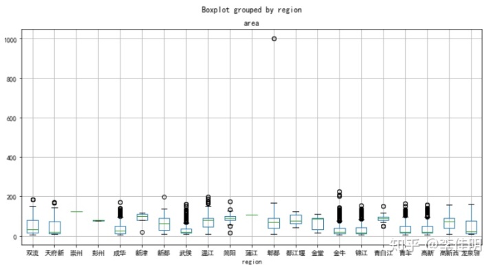

从图中可以看出，主城区面积的中位数普遍低于周边县区面积的中位数，这是由于主城区的用于居住的土地面积较小，人口较多，从而导致房屋面积较小。而对于周边县区，人口密度较小，用于居住的土地较多，从而使房屋的面积较大。

下面针对几个典型区域进行分析。

# 针对高新区进行分析
data_gaoxin = data_clean[data_clean.region=='高新']
area_divide = [1, 30, 50, 70, 90,1200]
area_cut = pd.cut(list(data_gaoxin['area']), area_divide)
area_cut_data = area_cut.describe()
area_cut_data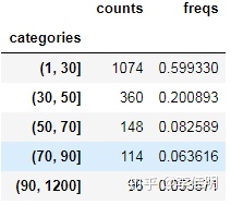

area_percentage = (area_cut_data['freqs'].values)*100
# 保留两位小数
np.set_printoptions(precision=2)
labels  = ['30平米以下', '30-50平米', '50-70平米', '70-90平米',
'90平米以上']
fig, axes = plt.subplots(figsize=(10,5),ncols=2) # 设置绘图区域大小
ax1, ax2 = axes.ravel()
patches, texts, autotexts = ax1.pie(x=area_percentage, labels=labels, autopct='%.2f%%',
        shadow=False, startangle=90)
ax1.axis('equal')  
ax1.set_title('高新区房源面积分布', loc='center')
# ax2 只显示图例（legend）
ax2.axis('off')
ax2.legend(patches, labels, loc='center left')
plt.tight_layout()
plt.show()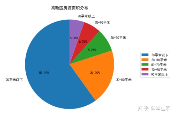

从图中看出，高新区的房源仍以30平米以下的小户型为主。

# 针对郫都区进行分析
data_pidu = data_clean[data_clean.region=='郫都']
area_divide = [1, 30, 50, 70, 90,1200]
area_cut = pd.cut(list(data_pidu['area']), area_divide)
area_cut_data = area_cut.describe()
area_cut_data

area_percentage = (area_cut_data['freqs'].values)*100
# 保留两位小数
np.set_printoptions(precision=2)
labels  = ['30平米以下', '30-50平米', '50-70平米', '70-90平米',
'90平米以上']
fig, axes = plt.subplots(figsize=(10,5),ncols=2) # 设置绘图区域大小
ax1, ax2 = axes.ravel()
patches, texts, autotexts = ax1.pie(x=area_percentage, labels=labels, autopct='%.2f%%',
        shadow=False, startangle=90)
ax1.axis('equal')  
ax1.set_title('郫都区房源面积分布', loc='center')
# ax2 只显示图例（legend）
ax2.axis('off')
ax2.legend(patches, labels, loc='center left')
plt.tight_layout()
plt.show()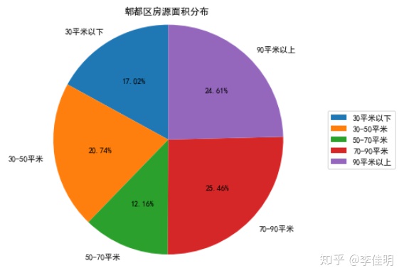

从图中可以看出，郫都区70平米以上的房源占到了50%，不再是小户型作为主要房源。

data_wj = data_clean[data_clean.region=='温江']
area_divide = [1, 30, 50, 70, 90,1200]
area_cut = pd.cut(list(data_wj['area']), area_divide)
area_cut_data = area_cut.describe()
area_cut_data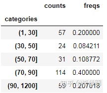

area_percentage = (area_cut_data['freqs'].values)*100
# 保留两位小数
np.set_printoptions(precision=2)
labels  = ['30平米以下', '30-50平米', '50-70平米', '70-90平米',
'90平米以上']
fig, axes = plt.subplots(figsize=(10,5),ncols=2) # 设置绘图区域大小
ax1, ax2 = axes.ravel()
patches, texts, autotexts = ax1.pie(x=area_percentage, labels=labels, autopct='%.2f%%',
        shadow=False, startangle=90)
ax1.axis('equal')  
ax1.set_title('温江区房源面积分布', loc='center')
# ax2 只显示图例（legend）
ax2.axis('off')
ax2.legend(patches, labels, loc='center left')
plt.tight_layout()
plt.show()

从图中可以看出，温江区70平米以上的房源占比达到了60%以上，房源平均面积进一步提升。

4.总结

1、成都市的五大主城区和高新区有着大量的房源，并且高新区房源最多。此外郫都区、温江区和龙泉驿区等地区也有着大量房源，在租房时可在上述区域优先选择。

2、就价格而言，绝大部分房租价格位于2000以下，最贵房租为9300。所有区域中，成华区、武侯区、金牛区、锦江区、青羊区和高新区的房源平均价格远大于其他区域的价格，因为上述几区作为成都的主城区，租金相对其他区域自然偏高一些，而高新区的平均价格最高，可能是因为人口较多，经济发达导致的。

3、成都市的房源整体上以30平米以下的小户型为主，但不同区域也存在一定的差别。比如高新区30平米以下房源的比例接近60%，超过了整体上房源中的比例；郫都区和温江区等区域，主要以70平米以上的户型为主。房源面积分布按照地理位置呈现出了差异。

4、对于寻求较低租赁价格和较大房屋面积的租户，可考虑在周边县区进行寻找；对于出租人来说，在主城区推出小户型的房源，会更受市场青睐。