hough变换_如何用霍夫变换算法实现直线检测

原文最初发表于 Medium 博客，经原作者 Socret Lee 授权，InfoQ 中文站翻译并分享。

导读：如果告诉你一张图里面有一条看起来挺直的线，让你指出来线在哪、线的指向是向哪个方向。你肯定可以不假思索地告诉我线的位置和方向。但这个任务对计算机来说，可不是一件简单的事，因为图片在计算机中的存储形式就是 0001101111001010110101…，根本没有办法从这个序列中直接给出是否有直线以及直线的位置。要怎么才能让计算机自己学会找直线呢？这就要用霍夫变换了。霍夫变换是一种特征提取，广泛应用于在图像分析、计算机视觉以及数字影像处理。霍夫变换是用来识别找出目标中的特征，例如线条。它的算法过程大致如下：给定一个对象，要辨别的形状的种类，算法会在参数空间中执行投票来决定对象的形状，而这是由累加空间里的局部最大值来决定。本文阐述了一种在图像中寻找直线的算法。

I. 动机

最近，我发现自己需要在一个 APP 中加入一个文档扫描功能。在做了一些研究之后，我偶然看到了 Dropbox 机器学习团队成员 Ying Xiong 写的一篇文章《快速、准确的扫描文档检测》(Fast and Accurate Document Detection for Scanning)。这篇文章解释了 Dropbox 机器学习团队如何实现文档扫描的功能，并重点介绍了他们所经历的步骤和每一步所使用的算法。正是通过这篇文章，我了解到一种叫做霍夫变换(Hough Transform)的算法，以及如何利用霍夫变换来检测图像中的直线。因此，在本文中，我想讲解一下霍夫变换算法，并提供霍夫变换算法在 Python 中的“从头开始”实现。

II. 霍夫变换

霍夫变换是 Paul V.C. Hough 在 1962 年申请为专利的一种算法，最初是为了识别照片中的复杂线条而发明的。自该算法发明以来，经过不断的修改和增强，现在已经能够识别其他形状，如圆形和四边形等特定类型的形状。为了了解霍夫变换算法的工作原理，就必须了解这四个概念：边缘图像、霍夫空间和边缘点到霍夫空间的映射、表示直线的另一种方式，以及如何检测直线。

边缘图像

Canny 边缘检测算法。来源： https://aishack.in/tutorials/canny-edge-detector/

边缘图像是边缘检测算法的输出。边缘检测算法通过确定图像的亮度或强度急剧变化的位置来检测图像中的边缘(摘自《边缘检测：用 Python 进行图像处理》(Edge Detection — Image Processing with Python)，2020 年)。边缘检测算法的示例包括： Canny 、 Sobel 、 Laplacian 等。通常边缘图像是二值化的，二值化意味着图像所有的像素都是 1 或 0。对于霍夫变换算法，关键是首先要进行边缘检测，以生成边缘图像，然后将其作为算法的输入。

霍夫空间与边缘点到霍夫空间的映射

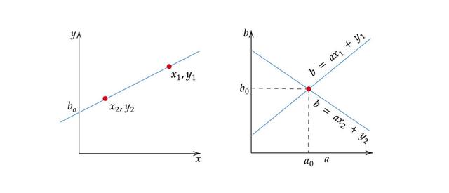
从边缘点到霍夫空间的映射

霍夫空间是一个二维平面，其中横轴表示斜率，纵轴表示直线在边缘图像上的截距。边缘图像上的线以 y=ax+by=ax+b 的形式表示。边缘图像上的一条线在霍夫空间上产生一个点，因为一条线的特征是其斜率为 aa，截距为 bb。另一方面，边缘图像上的边缘点 (xi,yi)(xi,yi)，可以有无限多条线穿过它。因此，一个边缘点在霍夫空间中以 b=axi+yib=axi+yi 的形式产生一条线。在霍夫变换算法中，霍夫空间用于确定边缘图像是否存在直线。

表示直线的另一种方式

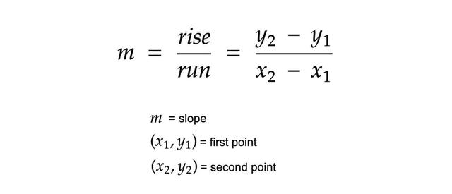
用于计算直线斜率的方程式

用 y=ax+by=ax+b 的形式来表示直线，用斜率和截距表示霍夫空间，这种方法存在一个缺陷。在这种形式下，该算法将无法检测出垂直线，因为对于垂直线来说，斜率 aa 是不确定的 / 无穷大。从编程的角度来说，这意味着计算机需要无限数量的内存来表示 aa 的所有可能值。为避免出现这个问题，直线改为由一条称为法线的直线表示，这条线穿过原点并垂直于这条直线。法线的形式为 ρ=xcos(θ)+ysin(θ)ρ=xcos⁡(θ)+ysin⁡(θ)，其中，ρρ 是法线的长度，θθ 是法线与 x 轴之间的夹角。

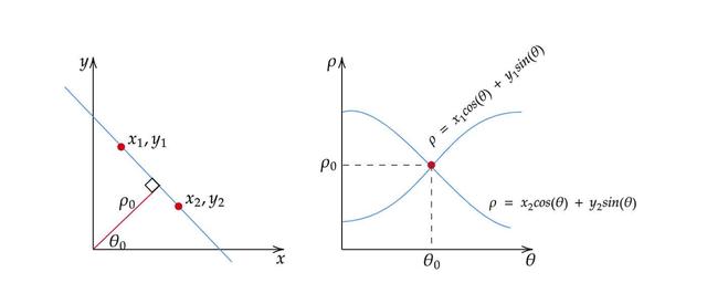
直线的另一种表示及其对应的霍夫空间

使用这个方法，不再用斜率 aa 和截距 bb 来表示霍夫空间，而是用 ρρ 和 θθ 表示，其中横轴为 θθ 值，纵轴为 ρρ 值。边缘点映射到霍夫空间的工作原理与此类似，只是边缘点 (xi,yi)(xi,yi) 现在在霍夫空间生成的是余弦曲线而不是直线。这种正常的直线表示法消除了在处理垂直线时出现的 aa 的无界值的问题。

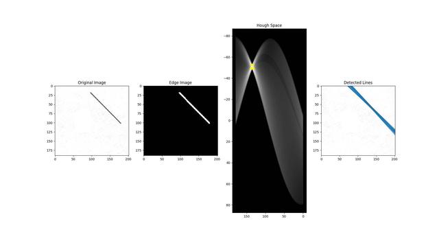
直线检测

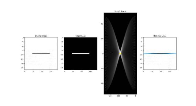
在图像中检测直线的过程。护肤空间中的黄点表示直线存在，并由 θ 和 ρ 对表示

如前所述，边缘点在霍夫空间中产生了余弦曲线。由此，如果我们将所有的边缘点从边缘图像映射到霍夫空间，它将产生大量的余弦曲线。如果两遍边缘点位于同一直线上，则它们对应的余弦曲线将在特定的 (ρ,θ)(ρ,θ) 对上彼此相交。因此，霍夫变换算法是通过查找交叉点数量大于某一阈值的 (ρ,θ)(ρ,θ) 对来检测直线。值得注意的是，如果不进行一些预处理的话，比如在霍夫空间上进行邻域抑制，以去除边缘图像中类似的直线，这种阈值的方法可能不一定能得到最好的结果。

III. 算法

1. 确定 ρρ 和 θθ 的范围。通常，θθ 的范围为 0,1800,180，其中 dd 是边缘图像的对角线的长度。重要的是要对 ρρ 和 θθ 的范围进行量化，这意味着这一范围的可能值的数量应该是有限的。
2. 创建一个名为累加器的二维数组，该数组表示具有维数 (numrhos,numthetas)(numrhos,numthetas) 的霍夫空间，并将其所有制初始化为零。
3. 对原始图像进行边缘检测。这可以用你选择的任何边缘检测算法来完成。
4. 对于边缘图像上的每个像素，检查改像素是否为边缘像素。如果是边缘像素，则循环遍历 θθ 的所有可能值，计算相应的 ρρ ，在累加器中找到 ρρ 和 θθ 的索引，并基于这些索引对递增累加器。
5. 循环遍历累加器中的所有制。如果该值大于某一阈值，则获取 ρρ 和 θθ 的索引，从索引对中获取 ρρ 和 θθ 的值，然后可以将其转换回 y=ax+by=ax+b 的形式。

IV. 代码实现

非向量化解决方案

复制代码

import cv2import numpy as npimport matplotlib.pyplot as pltimport matplotlib.lines as mlines def line_detection_non_vectorized(image, edge_image, num_rhos=180, num_thetas=180, t_count=220):  edge_height, edge_width = edge_image.shape[:2]  edge_height_half, edge_width_half = edge_height / 2, edge_width / 2  #  d = np.sqrt(np.square(edge_height) + np.square(edge_width))  dtheta = 180 / num_thetas  drho = (2 * d) / num_rhos  #  thetas = np.arange(0, 180, step=dtheta)  rhos = np.arange(-d, d, step=drho)  #  cos_thetas = np.cos(np.deg2rad(thetas))  sin_thetas = np.sin(np.deg2rad(thetas))  #  accumulator = np.zeros((len(rhos), len(rhos)))  #  figure = plt.figure(figsize=(12, 12))  subplot1 = figure.add_subplot(1, 4, 1)  subplot1.imshow(image)  subplot2 = figure.add_subplot(1, 4, 2)  subplot2.imshow(edge_image, cmap="gray")  subplot3 = figure.add_subplot(1, 4, 3)  subplot3.set_facecolor((0, 0, 0))  subplot4 = figure.add_subplot(1, 4, 4)  subplot4.imshow(image)  #  for y in range(edge_height):    for x in range(edge_width):      if edge_image[y][x] != 0:        edge_point = [y - edge_height_half, x - edge_width_half]        ys, xs = [], []        for theta_idx in range(len(thetas)):          rho = (edge_point[1] * cos_thetas[theta_idx]) + (edge_point[0] * sin_thetas[theta_idx])          theta = thetas[theta_idx]          rho_idx = np.argmin(np.abs(rhos - rho))          accumulator[rho_idx][theta_idx] += 1          ys.append(rho)          xs.append(theta)        subplot3.plot(xs, ys, color="white", alpha=0.05)  for y in range(accumulator.shape[0]):    for x in range(accumulator.shape[1]):      if accumulator[y][x] > t_count:        rho = rhos[y]        theta = thetas[x]        a = np.cos(np.deg2rad(theta))        b = np.sin(np.deg2rad(theta))        x0 = (a * rho) + edge_width_half        y0 = (b * rho) + edge_height_half        x1 = int(x0 + 1000 * (-b))        y1 = int(y0 + 1000 * (a))        x2 = int(x0 - 1000 * (-b))        y2 = int(y0 - 1000 * (a))        subplot3.plot([theta], [rho], marker='o', color="yellow")        subplot4.add_line(mlines.Line2D([x1, x2], [y1, y2]))  subplot3.invert_yaxis()  subplot3.invert_xaxis()  subplot1.title.set_text("Original Image")  subplot2.title.set_text("Edge Image")  subplot3.title.set_text("Hough Space")  subplot4.title.set_text("Detected Lines")  plt.show()  return accumulator, rhos, thetas if __name__ == "__main__":  for i in range(3):    image = cv2.imread(f"sample-{i+1}.png")    edge_image = cv2.cvtColor(image, cv2.COLOR_BGR2GRAY)    edge_image = cv2.GaussianBlur(edge_image, (3, 3), 1)    edge_image = cv2.Canny(edge_image, 100, 200)    edge_image = cv2.dilate(        edge_image,        cv2.getStructuringElement(cv2.MORPH_RECT, (5, 5)),        iterations=1    )    edge_image = cv2.erode(        edge_image,        cv2.getStructuringElement(cv2.MORPH_RECT, (5, 5)),        iterations=1    )    line_detection_non_vectorized(image, edge_image)

向量化解决方案

复制代码

import cv2import numpy as npimport matplotlib.pyplot as pltimport matplotlib.lines as mlines def line_detection_vectorized(image, edge_image, num_rhos=180, num_thetas=180, t_count=220):  edge_height, edge_width = edge_image.shape[:2]  edge_height_half, edge_width_half = edge_height / 2, edge_width / 2  #  d = np.sqrt(np.square(edge_height) + np.square(edge_width))  dtheta = 180 / num_thetas  drho = (2 * d) / num_rhos  #  thetas = np.arange(0, 180, step=dtheta)  rhos = np.arange(-d, d, step=drho)  #  cos_thetas = np.cos(np.deg2rad(thetas))  sin_thetas = np.sin(np.deg2rad(thetas))  #  accumulator = np.zeros((len(rhos), len(rhos)))  #  figure = plt.figure(figsize=(12, 12))  subplot1 = figure.add_subplot(1, 4, 1)  subplot1.imshow(image)  subplot2 = figure.add_subplot(1, 4, 2)  subplot2.imshow(edge_image, cmap="gray")  subplot3 = figure.add_subplot(1, 4, 3)  subplot3.set_facecolor((0, 0, 0))  subplot4 = figure.add_subplot(1, 4, 4)  subplot4.imshow(image)  #  edge_points = np.argwhere(edge_image != 0)  edge_points = edge_points - np.array([[edge_height_half, edge_width_half]])  #  rho_values = np.matmul(edge_points, np.array([sin_thetas, cos_thetas]))  #  accumulator, theta_vals, rho_vals = np.histogram2d(      np.tile(thetas, rho_values.shape[0]),      rho_values.ravel(),      bins=[thetas, rhos]  )  accumulator = np.transpose(accumulator)  lines = np.argwhere(accumulator > t_count)  rho_idxs, theta_idxs = lines[:, 0], lines[:, 1]  r, t = rhos[rho_idxs], thetas[theta_idxs]  for ys in rho_values:    subplot3.plot(thetas, ys, color="white", alpha=0.05)  subplot3.plot([t], [r], color="yellow", marker='o')  for line in lines:    y, x = line    rho = rhos[y]    theta = thetas[x]    a = np.cos(np.deg2rad(theta))    b = np.sin(np.deg2rad(theta))    x0 = (a * rho) + edge_width_half    y0 = (b * rho) + edge_height_half    x1 = int(x0 + 1000 * (-b))    y1 = int(y0 + 1000 * (a))    x2 = int(x0 - 1000 * (-b))    y2 = int(y0 - 1000 * (a))    subplot3.plot([theta], [rho], marker='o', color="yellow")    subplot4.add_line(mlines.Line2D([x1, x2], [y1, y2]))  subplot3.invert_yaxis()  subplot3.invert_xaxis()  subplot1.title.set_text("Original Image")  subplot2.title.set_text("Edge Image")  subplot3.title.set_text("Hough Space")  subplot4.title.set_text("Detected Lines")  plt.show()  return accumulator, rhos, thetas if __name__ == "__main__":  for i in range(3):    image = cv2.imread(f"sample-{i+1}.png")    edge_image = cv2.cvtColor(image, cv2.COLOR_BGR2GRAY)    edge_image = cv2.GaussianBlur(edge_image, (3, 3), 1)    edge_image = cv2.Canny(edge_image, 100, 200)    edge_image = cv2.dilate(        edge_image,        cv2.getStructuringElement(cv2.MORPH_RECT, (5, 5)),        iterations=1    )    edge_image = cv2.erode(        edge_image,        cv2.getStructuringElement(cv2.MORPH_RECT, (5, 5)),        iterations=1    )    line_detection_vectorized(image, edge_image)

V. 结论

最后，本文以最简单的形式介绍了霍夫变换算法。如前所述，该算法可以扩展到直线检测之外。多年来，这种算法得到了许多改进，现在能够检测其他形状了，如圆形、三角形，甚至是特定形状的四边形等。由此产生了许多有用的现实世界应用，从文档扫描到自动驾驶汽车的车道检测。我相信，在可预见的未来，还会有更多令人惊叹的技术在这一算法的推动下问世。

参考文献

• 《边缘检测：用 Python 进行图像处理》(Edge Detection — Image Processing with Python.)(2020 年 2 月 16 日)
• 《辨识复杂图案的方法及手段》(Method and means for recognizing complex patterns) Hough, P.V.C.(1962 年)
• 《 v 》(Tutorial: Build a lane detector. Towards Data Science.">教程：构建车道检测器 Lin, C(2018 年 12 月 17 日)
• 《霍夫变换综述与模式识别》(A survey of Hough Transform. Pattern Recognition.)，Mukhopadhyay, P., 与 Chaudhuria, B. B. (2015 年)
• 《用 ImageJ 进行霍夫圆变换》(Hough Circle Transform. ImageJ.)Smith, B.(2018 年 9 月 21 日)
• 《 Sobel 边缘检测算法的实现》(An Implementation of Sobel Edge Detection.)Sodha, S.(2017 年)
• 《霍夫变换》(The Hough Transform)
• 《快速准确的扫描文档检测》( Fast and Accurate Document Detection for Scanning.) Xiong,Y.(2016 年)