dataframe切片_Kaggle：识别淋巴结病理切片有无癌细胞（logistic+svm+rf+CNN）

介绍

• 目的：识别淋巴结病理切片有无癌细胞
• 数据：Histopathologic Cancer Detection（鉴别淋巴结病理切片有无癌细胞），为图像二分类数据集 (图片大小
  )，来自
  Kaggle，可下载；为减少运算时间，仅使用 220025 张训练集中的 12000 张图片用于分析（已知标签），划分训练集（8000 张）、验证集（2000 张）和测试集（2000 张）；训练集用于建模，验证集用于超参数调优，测试集用于评价模型预测效果
• 预测模型：Logistic、SVM、RandomForest、CNN（基于 keras）
• 预测效果指标：准确率和 ROC 曲线下面积 AUC

使用的 Python 库

import numpy as np
import pandas as pd 
import matplotlib.pyplot as plt
import os
import warnings
from glob import glob
from PIL import Image

from sklearn.preprocessing import MinMaxScaler
from sklearn.linear_model import LogisticRegression
from sklearn.svm import SVC
from sklearn.ensemble import RandomForestClassifier
from sklearn.model_selection import train_test_split, KFold, GridSearchCV
from sklearn.metrics import roc_curve, auc, accuracy_score

warnings.filterwarnings("ignore")
os.chdir("D:/BigData/histopathologic-cancer-detection")

from IPython.core.interactiveshell import InteractiveShell
InteractiveShell.ast_node_interactivity = "all"

定义 ROC 曲线绘制函数

def plot_roc(y_true, y_pred, predict_prob, label = ""):
    FP, TP, thresholds = roc_curve(y_true, predict_prob)
    roc_auc = auc(FP, TP)
    acc = accuracy_score(y_true, y_pred)
    plt.style.use("ggplot")
    plt.figure(dpi = 120)
    plt.plot(FP, TP, color = "blue")
    plt.plot([0, 1], [0, 1], "r--")
    plt.title(label + " AUC")
    plt.xlabel("FP")
    plt.ylabel("TP")
    plt.text(0.6, 0.35, "AUC = %.3fnAccuracy = %.3f" % (roc_auc, acc))
    plt.show;

读入、查看数据

train 文件夹内是已知标签的病理图片，图片名与 train_labels.csv 文件的 id 变量对应，label 变量表示有无癌细胞

训练集共有 220025 张图片

labels_df = pd.read_csv("train_labels.csv")
labels_df.shape
print(labels_df.head())

(220025, 2)

                                         id  label
0  f38a6374c348f90b587e046aac6079959adf3835      0
1  c18f2d887b7ae4f6742ee445113fa1aef383ed77      1
2  755db6279dae599ebb4d39a9123cce439965282d      0
3  bc3f0c64fb968ff4a8bd33af6971ecae77c75e08      0
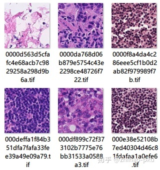
4  068aba587a4950175d04c680d38943fd488d6a9d      0

读取 train 文件内所有图片的路径为 path 变量

imgs_path_df = pd.DataFrame(glob("train/*.tif"), columns = ["path"])
imgs_path_df["id"] = imgs_path_df["path"].map(lambda x: x.split("")[-1].split(".")[0])
imgs_path_df.shape
print(imgs_path_df.head())

(220025, 2)

                                                path  
0  train00001b2b5609af42ab0ab276dd4cd41c3e7745b5...   
1  train000020de2aa6193f4c160e398a8edea95b1da598...   
2  train00004aab08381d25d315384d646f5ce413ea24b1...   
3  train0000d563d5cfafc4e68acb7c9829258a298d9b6a...   
4  train0000da768d06b879e5754c43e2298ce48726f722...   

                                         id  
0  00001b2b5609af42ab0ab276dd4cd41c3e7745b5  
1  000020de2aa6193f4c160e398a8edea95b1da598  
2  00004aab08381d25d315384d646f5ce413ea24b1  
3  0000d563d5cfafc4e68acb7c9829258a298d9b6a  
4  0000da768d06b879e5754c43e2298ce48726f722

将图片路径与图片标签 merge 起来

df = pd.merge(imgs_path_df, labels_df, on = "id", how = "left")
df.shape
print(df.head())

(220025, 3)

                                                path  
0  train00001b2b5609af42ab0ab276dd4cd41c3e7745b5...   
1  train000020de2aa6193f4c160e398a8edea95b1da598...   
2  train00004aab08381d25d315384d646f5ce413ea24b1...   
3  train0000d563d5cfafc4e68acb7c9829258a298d9b6a...   
4  train0000da768d06b879e5754c43e2298ce48726f722...   

                                         id  label  
0  00001b2b5609af42ab0ab276dd4cd41c3e7745b5      1  
1  000020de2aa6193f4c160e398a8edea95b1da598      0  
2  00004aab08381d25d315384d646f5ce413ea24b1      0  
3  0000d563d5cfafc4e68acb7c9829258a298d9b6a      0  
4  0000da768d06b879e5754c43e2298ce48726f722      1

选取训练集 220025 张图片中的 12000 张用于后续分析；8000 张作为训练集，2000 张作为验证集，2000 张作为测试集

index = np.random.permutation(df.shape[0])
df = df.iloc[index]

train, valid = train_test_split(df[:10000], test_size = 0.2, stratify = df[:10000]["label"], random_state = 0)
test = df.iloc[10000:12000]

print("训练集图片数：" + str(train.shape[0]))
print("验证集图片数：" + str(valid.shape[0]))
print("测试集图片数：" + str(test.shape[0]))

# 12000张图片中0、1结局的比例
df[:12000]["label"].value_counts(normalize=True)

训练集图片数：8000
验证集图片数：2000
测试集图片数：2000

0    0.594917
1    0.405083
Name: label, dtype: float64
print("图像大小为：" + str(np.asarray(Image.open(df.iloc[0]["path"])).shape))

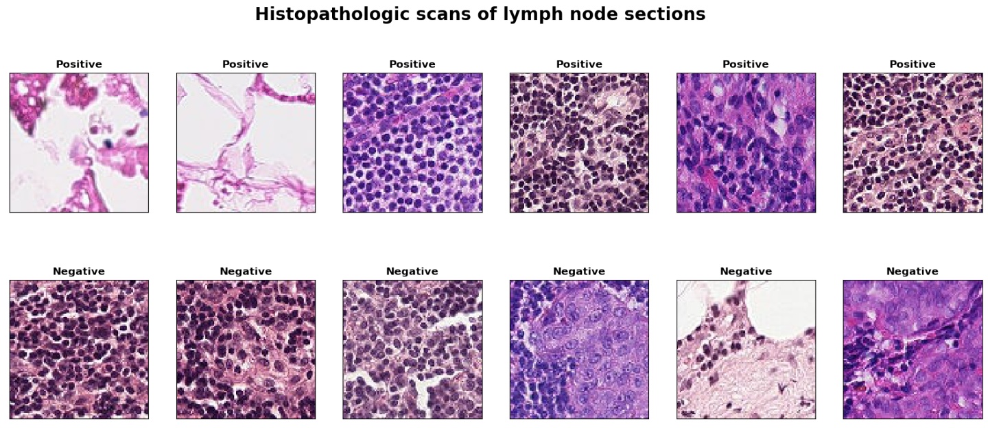
图像大小为：(96, 96, 3)

分别展示 6 张有癌细胞的图片（Positive）和没有癌细胞的图片（Negative）

df1 = df[df["label"] == 1]
df2 = df[df["label"] == 0]

fig, ax = plt.subplots(2, 6, figsize = (20, 8), dpi = 100)
fig.suptitle("Histopathologic scans of lymph node sections", fontsize = 20, fontweight = "bold")

random_num1 = list(np.random.randint(0, df1.shape[0] - 1, size = 6))
random_num2 = list(np.random.randint(0, df2.shape[0] - 1, size = 6))

for i, j in enumerate(zip(random_num1, random_num2)):
    j1, j2 = j
    ax[0, i].imshow(np.asarray(Image.open(df.iloc[j1]["path"])))
    ax[0, i].set_xticks([])
    ax[0, i].set_yticks([])
    ax[0, i].set_title("Positive", fontweight = "bold")
    
    ax[1, i].imshow(np.asarray(Image.open(df.iloc[j2]["path"])))
    ax[1, i].set_xticks([])
    ax[1, i].set_yticks([])
    ax[1, i].set_title("Negative", fontweight = "bold")

plt.show();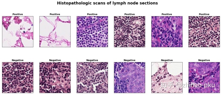

Logistic、SVM、RandomForest 建模

数据预处理

读入所有图片为数组；压缩图片大小，由 [96, 96, 3] 转为 [24, 24, 3]

train_imgs = np.ndarray((train.shape[0], 24, 24, 3))
train_labels = np.ndarray((train.shape[0], ))

valid_imgs = np.ndarray((valid.shape[0], 24, 24, 3))
valid_labels = np.ndarray((valid.shape[0], ))

test_imgs = np.ndarray((test.shape[0], 24, 24, 3))
test_labels = np.ndarray((test.shape[0], ))

for i, j in enumerate(train["path"]):
    img = np.asarray(Image.open(j).resize((24, 24)))
    train_imgs[i] = img
    train_labels[i] = train["label"].iloc[i]

for i, j in enumerate(valid["path"]):
    img = np.asarray(Image.open(j).resize((24, 24)))
    valid_imgs[i] = img
    valid_labels[i] = valid["label"].iloc[i]
    
for i, j in enumerate(test["path"]):
    img = np.asarray(Image.open(j).resize((24, 24)))
    test_imgs[i] = img
    test_labels[i] = test["label"].iloc[i]

将数组形状由 [*, 24, 24, 3] 转变为 [*,

]，以用于 Logistic、SVM、RandomForest 建模

# 最小最大标准化
scaler = MinMaxScaler()

train_x = train_imgs.reshape(-1, 24 * 24 * 3)
scaler.fit(train_x)
train_x = scaler.transform(train_x)
train_y = train_labels

valid_x = valid_imgs.reshape(-1, 24 * 24 * 3)
valid_x = scaler.transform(valid_x)
valid_y = valid_labels

test_x = test_imgs.reshape(-1, 24 * 24 * 3)
test_x = scaler.transform(test_x)
test_y = test_labels

train_x.shape
train_y.shape

valid_x.shape
valid_y.shape

test_x.shape
test_y.shape

MinMaxScaler(copy=True, feature_range=(0, 1))


(8000, 1728)


(8000,)


(2000, 1728)


(2000,)


(2000, 1728)


(2000,)

logistic 结果

%%time

logit = LogisticRegression()
logit.fit(train_x, train_y)

y_pred = logit.predict(test_x)
y_prob = logit.predict_proba(test_x)
plot_roc(test_y, y_pred, y_prob[:, 1], label = "LogisticRegression")

Wall time: 1.39 s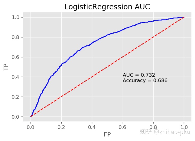

SVM 结果

%%time

svc = SVC(probability = True)
svc.fit(train_x, train_y)

y_pred = svc.predict(test_x)
y_prob = svc.predict_proba(test_x)
plot_roc(test_y, y_pred, y_prob[:, 1], label = "SVC")

Wall time: 10min 4s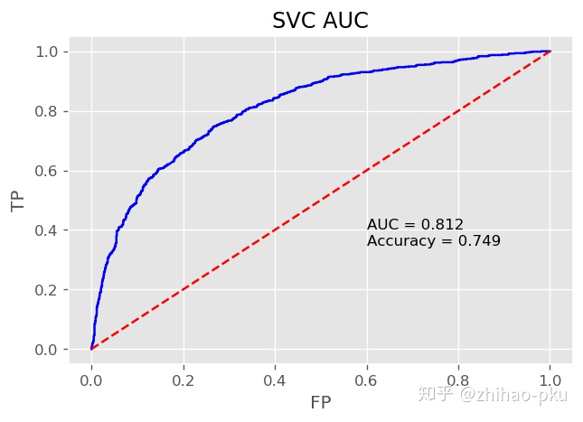

RandomForest 结果

%%time

rf = RandomForestClassifier()
rf.fit(train_x, train_y)

y_pred = rf.predict(test_x)
y_prob = rf.predict_proba(test_x)
plot_roc(test_y, y_pred, y_prob[:, 1], label = "RandomForest")

Wall time: 21.9 s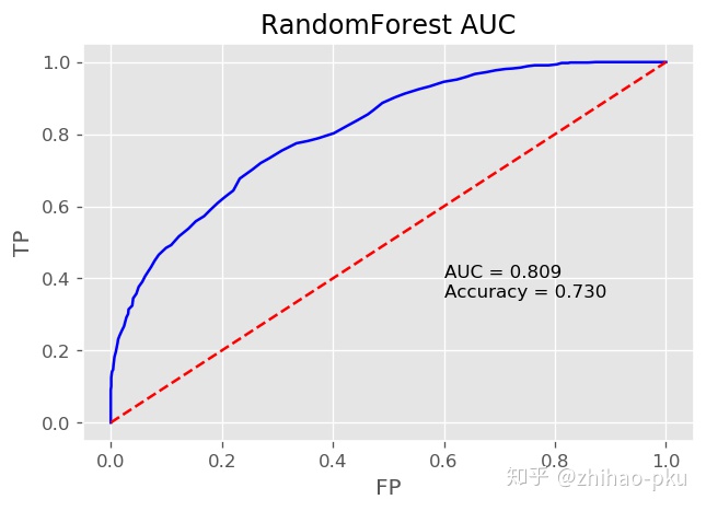

使用网格搜索和 3 折交叉验证选择 RandomForest 超参数：分类树数量和最小叶节点数；共需要拟合

个模型

%%time

kfold = KFold(n_splits=3, random_state=0)
rf_param_grid = {"n_estimators": [100, 300],
                 "min_samples_leaf": [1, 3, 10]}

gsrf = GridSearchCV(RandomForestClassifier(), param_grid=rf_param_grid, 
                    cv=kfold, scoring="accuracy", 
                    n_jobs= 4, verbose = 1)

gsrf.fit(np.concatenate([train_x, valid_x], axis=0), np.concatenate([train_y, valid_y], axis=0))
rf_best = gsrf.best_estimator_

Fitting 3 folds for each of 6 candidates, totalling 18 fits


[Parallel(n_jobs=4)]: Using backend LokyBackend with 4 concurrent workers.
[Parallel(n_jobs=4)]: Done  18 out of  18 | elapsed:  4.0min finished


Wall time: 5min 17s

使用网格搜索选出的最优 RandomForest 对测试集进行预测

y_pred = rf_best.predict(test_x)
y_prob = rf_best.predict_proba(test_x)
plot_roc(test_y, y_pred, y_prob[:, 1], label = "RandomForest")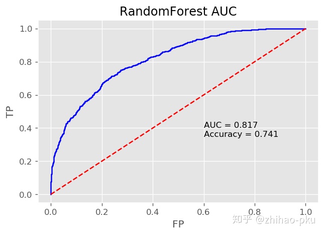

三个模型小结

• 明显看出 Logistic 分类效果在三者中最差，不再考虑对它进行超参数调优；建立单个模型所用时间，SVM（RBF 核）最长；RandomForest 预测效果略微差于 SVM，且训练时间较短，因此对它进行超参数调优
• LogisticRegression 预测准确率为：0.69，ROC 曲线下面积 AUC 为：0.73
• SVC with RBF kernel 预测准确率为：0.75，ROC 曲线下面积 AUC 为：0.81
• RandomForest 调优前预测准确率为：0.73，ROC 曲线下面积 AUC 为：0.81；调优后为 0.74 和 0.82

卷积神经网络（CNN）建模

from keras.preprocessing.image import ImageDataGenerator
from keras.models import Sequential
from keras.layers import Dense, Dropout, Flatten, BatchNormalization, Activation
from keras import optimizers
from keras.applications.vgg19 import VGG19
from keras.callbacks import EarlyStopping, ReduceLROnPlateau
from keras import backend as K

Using TensorFlow backend.
train["label"] = train["label"].astype(str)
valid["label"] = valid["label"].astype(str)
test["label"] = test["label"].astype(str)

构建数据生成器，分批次将数据读入 CNN 训练

# 像素值归一化到0-1，同时使用水平、垂直、旋转、缩放变换等数据增强方法
train_datagen = ImageDataGenerator(
    rescale = 1 / 255,
    vertical_flip = True,
    horizontal_flip = True,
    rotation_range = 90,
    zoom_range = 0.2, 
    width_shift_range = 0.1,
    height_shift_range = 0.1,
    shear_range = 0.05,
    channel_shift_range = 0.1
)

# 按照train数据框的图片路径和标签分批次读入数据
train_generator = train_datagen.flow_from_dataframe(
    dataframe = train, 
    directory = None, 
    x_col = "path", 
    y_col = "label", 
    target_size = (96, 96), 
    class_mode = "binary", 
    batch_size = 64, 
    seed = 0, 
    shuffle = True
)

valid_datagen = ImageDataGenerator(
    rescale = 1 / 255
)

valid_generator = valid_datagen.flow_from_dataframe(
    dataframe = valid, 
    directory = None, 
    x_col = "path", 
    y_col = "label", 
    target_size = (96, 96), 
    class_mode = "binary", 
    batch_size = 64, 
    seed = 0, 
    shuffle = False
)

test_datagen = ImageDataGenerator(
    rescale = 1 / 255
)

test_generator = valid_datagen.flow_from_dataframe(
    dataframe = test, 
    directory = None, 
    x_col = "path", 
    y_col = "label", 
    target_size = (96, 96), 
    class_mode = "binary", 
    batch_size = 64, 
    seed = 0, 
    shuffle = False
)

Found 8000 validated image filenames belonging to 2 classes.
Found 2000 validated image filenames belonging to 2 classes.
Found 2000 validated image filenames belonging to 2 classes.

使用预训练的 VGG19，在该数据集上微调

K.clear_session()

# 在imagenet数据集上训练的VGG19，去掉顶端的全连接网络
vgg_conv_base = VGG19(weights = "imagenet", include_top = False, input_shape = (96, 96, 3))

vgg = Sequential()
vgg.add(vgg_conv_base)
vgg.add(Flatten())
vgg.add(Dense(128, use_bias = False))
vgg.add(BatchNormalization())
vgg.add(Activation("relu"))
vgg.add(Dropout(0.5))
vgg.add(Dense(1, activation = "sigmoid"))

查看网络结构

vgg_conv_base.summary()

Model: "vgg19"
_________________________________________________________________
Layer (type)                 Output Shape              Param #   
=================================================================
input_1 (InputLayer)         (None, 96, 96, 3)         0         
_________________________________________________________________
block1_conv1 (Conv2D)        (None, 96, 96, 64)        1792      
_________________________________________________________________
block1_conv2 (Conv2D)        (None, 96, 96, 64)        36928     
_________________________________________________________________
block1_pool (MaxPooling2D)   (None, 48, 48, 64)        0         
_________________________________________________________________
block2_conv1 (Conv2D)        (None, 48, 48, 128)       73856     
_________________________________________________________________
block2_conv2 (Conv2D)        (None, 48, 48, 128)       147584    
_________________________________________________________________
block2_pool (MaxPooling2D)   (None, 24, 24, 128)       0         
_________________________________________________________________
block3_conv1 (Conv2D)        (None, 24, 24, 256)       295168    
_________________________________________________________________
block3_conv2 (Conv2D)        (None, 24, 24, 256)       590080    
_________________________________________________________________
block3_conv3 (Conv2D)        (None, 24, 24, 256)       590080    
_________________________________________________________________
block3_conv4 (Conv2D)        (None, 24, 24, 256)       590080    
_________________________________________________________________
block3_pool (MaxPooling2D)   (None, 12, 12, 256)       0         
_________________________________________________________________
block4_conv1 (Conv2D)        (None, 12, 12, 512)       1180160   
_________________________________________________________________
block4_conv2 (Conv2D)        (None, 12, 12, 512)       2359808   
_________________________________________________________________
block4_conv3 (Conv2D)        (None, 12, 12, 512)       2359808   
_________________________________________________________________
block4_conv4 (Conv2D)        (None, 12, 12, 512)       2359808   
_________________________________________________________________
block4_pool (MaxPooling2D)   (None, 6, 6, 512)         0         
_________________________________________________________________
block5_conv1 (Conv2D)        (None, 6, 6, 512)         2359808   
_________________________________________________________________
block5_conv2 (Conv2D)        (None, 6, 6, 512)         2359808   
_________________________________________________________________
block5_conv3 (Conv2D)        (None, 6, 6, 512)         2359808   
_________________________________________________________________
block5_conv4 (Conv2D)        (None, 6, 6, 512)         2359808   
_________________________________________________________________
block5_pool (MaxPooling2D)   (None, 3, 3, 512)         0         
=================================================================
Total params: 20,024,384
Trainable params: 20,024,384
Non-trainable params: 0
_________________________________________________________________
vgg.summary()

Model: "sequential_1"
_________________________________________________________________
Layer (type)                 Output Shape              Param #   
=================================================================
vgg19 (Model)                (None, 3, 3, 512)         20024384  
_________________________________________________________________
flatten_1 (Flatten)          (None, 4608)              0         
_________________________________________________________________
dense_1 (Dense)              (None, 128)               589824    
_________________________________________________________________
batch_normalization_1 (Batch (None, 128)               512       
_________________________________________________________________
activation_1 (Activation)    (None, 128)               0         
_________________________________________________________________
dropout_1 (Dropout)          (None, 128)               0         
_________________________________________________________________
dense_2 (Dense)              (None, 1)                 129       
=================================================================
Total params: 20,614,849
Trainable params: 20,614,593
Non-trainable params: 256
_________________________________________________________________

冻结 block5_conv1 之前的网络参数

vgg_conv_base.Trainable = True
set_trainable = False

for layer in vgg_conv_base.layers:
    if layer.name == "block5_conv1":
        set_trainable = True
    if set_trainable:
        layer.trainable = True
    else:
        layer.trainable = False

训练模型，应用早期终止和学习率衰减方法

%%time

vgg.compile(optimizers.Adam(0.001), loss = "binary_crossentropy", metrics = ["accuracy"])

train_step_size = train_generator.n // train_generator.batch_size
valid_step_size = valid_generator.n // valid_generator.batch_size

earlystopper = EarlyStopping(monitor = "val_loss", patience = 3, verbose = 1, restore_best_weights = True)
reducelr = ReduceLROnPlateau(monitor = "val_loss", patience = 3, verbose = 1, factor = 0.1)

vgg_history = vgg.fit_generator(train_generator, steps_per_epoch = train_step_size, epochs = 10, 
                                validation_data = valid_generator, validation_steps = valid_step_size, 
                                callbacks = [reducelr, earlystopper], verbose = 1)

Epoch 1/10
125/125 [==============================] - 779s 6s/step - loss: 0.4983 - accuracy: 0.7831 - val_loss: 0.4028 - val_accuracy: 0.8322
Epoch 2/10
125/125 [==============================] - 761s 6s/step - loss: 0.4117 - accuracy: 0.8217 - val_loss: 0.3278 - val_accuracy: 0.8280
Epoch 3/10
125/125 [==============================] - 695s 6s/step - loss: 0.4045 - accuracy: 0.8271 - val_loss: 0.4262 - val_accuracy: 0.8275
Epoch 4/10
125/125 [==============================] - 672s 5s/step - loss: 0.3870 - accuracy: 0.8351 - val_loss: 0.2336 - val_accuracy: 0.8507
Epoch 5/10
125/125 [==============================] - 673s 5s/step - loss: 0.3771 - accuracy: 0.8414 - val_loss: 0.6309 - val_accuracy: 0.7552
Epoch 6/10
125/125 [==============================] - 679s 5s/step - loss: 0.3701 - accuracy: 0.8369 - val_loss: 0.2935 - val_accuracy: 0.8611
Epoch 7/10
125/125 [==============================] - 673s 5s/step - loss: 0.3598 - accuracy: 0.8491 - val_loss: 0.3296 - val_accuracy: 0.8600

Epoch 00007: ReduceLROnPlateau reducing learning rate to 0.00010000000474974513.
Restoring model weights from the end of the best epoch
Epoch 00007: early stopping
Wall time: 1h 22min 12s

CNN 结果

%%time

filenames = test_generator.filenames
labels = test_generator.labels

vgg_prob = vgg.predict_generator(test_generator).reshape(-1, )
vgg_pred = (vgg_prob > 0.5) * 1

res = pd.DataFrame(np.c_[filenames, vgg_prob, vgg_pred, labels], columns = ["filenames", "vgg_prob", "vgg_pred", "labels"])
res["vgg_prob"] = res["vgg_prob"].astype("float32")
res["vgg_pred"] = res["vgg_pred"].astype(int)
res["labels"] = res["labels"].astype(int)

Wall time: 1min 45s
print(res.head())

filenames  vgg_prob  vgg_pred  
0  traine4ed1411ec5ec20607f15e9c3c9c686bff222d23...  0.008025         0   
1  traincad3de976bdd02109f46030b412fb4aefecffde7...  0.039462         0   
2  train6f52280bab2dfe2b412f1e33f3b24b158cfdfd1c...  0.587529         1   
3  trainbdbb43f49991597f104da1c644ebbf184b3fc226...  0.034953         0   
4  train86d2d933c7ff35088d64fc85633d51598b713483...  0.992739         1   

   labels  
0       0  
1       0  
2       0  
3       0  
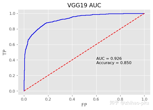
4       0

CNN 的预测准确率为：0.85，ROC 曲线下面积 AUC 为：0.93

plot_roc(res["labels"], res["vgg_pred"], res["vgg_prob"], label = "VGG19")

画出测试集的 6 张图片，标出真实标签和 CNN 的预测结果

labels_dict = {
    "1": "Positive", 
    "0": "Negative"
}

res["labels"] = res["labels"].astype(str).map(labels_dict)
res["vgg_pred"] = res["vgg_pred"].astype(str).map(labels_dict)

fig, ax = plt.subplots(1, 6, figsize = (20, 6), dpi = 100);
fig.suptitle("Histopathologic scans of lymph node sections", fontsize = 20, fontweight = "bold")

num_random = np.random.randint(0, res.shape[0] - 1, size = 6)  
  
for i, j in enumerate(num_random):
    ax[i].imshow(np.asarray(Image.open(res.iloc[j]["filenames"])))
    ax[i].set_xticks([])
    ax[i].set_yticks([])
    ax[i].set_title("Label: " + res.iloc[j]["labels"] + "n" + 
                    "Predictive: " + res.iloc[j]["vgg_pred"], fontweight = "bold")

plt.show();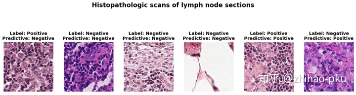

总结

• 使用 8000 张图片训练，在测试集上 CNN 的预测准确率和 ROC 曲线下面积均优于 Logistic、SVM、RandomForest
• 相比于预测准确率，ROC 曲线下面积更能代表一个预测模型的区分度：预测准确率受选定的概率 cutoff 值影响，选定不同的概率 cutoff 值就会产生不同的预测准确率；预测准确率在极度非平衡样本中是不可信的，比如数据中 99% 的个体为阳性，1% 为阴性，即使不建立预测模型，直接猜测所有个体为阳性，即可达到 0.99 的预测准确率；ROC 曲线下面积反映了预测模型在不同概率 cutoff 值下的综合预测能力，且在非平衡样本中依然可靠
• 如果有足够多的训练数据，甚至可以从头训练一个 CNN，其期预测能力会更佳