titanic数据集_10套练习，教你如何用Pandas做数据分析【6-10】

Pandas是入门Python做数据分析所必须要掌握的一个库，本文精选了十套练习题，帮助读者上手Python代码，完成数据集探索。

本文内容由科赛网翻译整理自Github，建议读者完成科赛网 从零上手Python关键代码 和 Pandas基础命令速查表 教程学习的之后，再对本教程代码进行调试学习。

【小提示：本文所使用的数据集下载地址：DATA | TRAIN 练习数据集】

一两赘肉无：10套练习，教你如何用Pandas做数据分析【1-5】​zhuanlan.zhihu.com

↓↓↓练习【6-10】↓↓↓

练习6-统计

探索风速数据

相应数据集：wind.data

步骤1 导入必要的库

# 运行以下代码
import pandas as pd
import datetime

步骤2 从以下地址导入数据

import pandas as pd
# 运行以下代码
path6 = "../input/pandas_exercise/exercise_data/wind.data"  # wind.data

步骤3 将数据作存储并且设置前三列为合适的索引

import datetime
# 运行以下代码
data = pd.read_table(path6, sep = "s+", parse_dates = [[0,1,2]]) 
data.head()

out[293]:

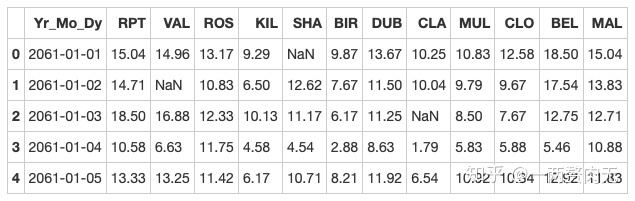
步骤4 2061年？我们真的有这一年的数据？创建一个函数并用它去修复这个bug

# 运行以下代码
def fix_century(x):
    year = x.year - 100 if x.year > 1989 else x.year
    return datetime.date(year, x.month, x.day)

# apply the function fix_century on the column and replace the values to the right ones
data['Yr_Mo_Dy'] = data['Yr_Mo_Dy'].apply(fix_century)

# data.info()
data.head()

out[294]:

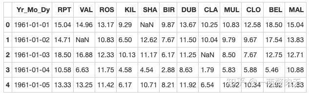
步骤5 将日期设为索引，注意数据类型，应该是datetime64[ns]

# 运行以下代码
# transform Yr_Mo_Dy it to date type datetime64
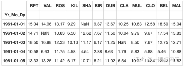
data["Yr_Mo_Dy"] = pd.to_datetime(data["Yr_Mo_Dy"])

# set 'Yr_Mo_Dy' as the index
data = data.set_index('Yr_Mo_Dy')

data.head()
# data.info() 

out[295]:

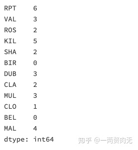
步骤6 对应每一个location，一共有多少数据值缺失

# 运行以下代码
data.isnull().sum()

out[296]:

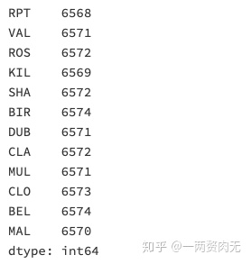
步骤7 对应每一个location，一共有多少完整的数据值

# 运行以下代码
data.shape[0] - data.isnull().sum()

out[297]:

步骤8 对于全体数据，计算风速的平均值

# 运行以下代码
data.mean().mean()

out[298]:

10.227982360836924

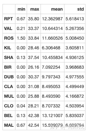
步骤9 创建一个名为loc_stats的数据框去计算并存储每个location的风速最小值，最大值，平均值和标准差

# 运行以下代码
loc_stats = pd.DataFrame()

loc_stats['min'] = data.min() # min
loc_stats['max'] = data.max() # max 
loc_stats['mean'] = data.mean() # mean
loc_stats['std'] = data.std() # standard deviations

loc_stats

out[299]:

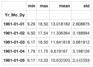
步骤10 创建一个名为day_stats的数据框去计算并存储所有location的风速最小值，最大值，平均值和标准差

# 运行以下代码
# create the dataframe
day_stats = pd.DataFrame()

# this time we determine axis equals to one so it gets each row.
day_stats['min'] = data.min(axis = 1) # min
day_stats['max'] = data.max(axis = 1) # max 
day_stats['mean'] = data.mean(axis = 1) # mean
day_stats['std'] = data.std(axis = 1) # standard deviations

day_stats.head()

out[300]:

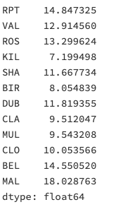
步骤11 对于每一个location，计算一月份的平均风速

(注意，1961年的1月和1962年的1月应该区别对待)

# 运行以下代码
# creates a new column 'date' and gets the values from the index
data['date'] = data.index

# creates a column for each value from date
data['month'] = data['date'].apply(lambda date: date.month)
data['year'] = data['date'].apply(lambda date: date.year)
data['day'] = data['date'].apply(lambda date: date.day)

# gets all value from the month 1 and assign to janyary_winds
january_winds = data.query('month == 1')

# gets the mean from january_winds, using .loc to not print the mean of month, year and day
january_winds.loc[:,'RPT':"MAL"].mean()

out[301]:

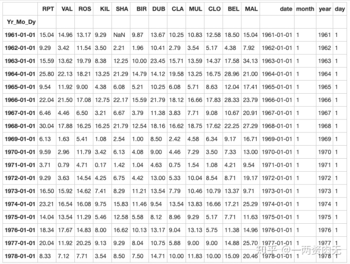
步骤12 对于数据记录按照年为频率取样

# 运行以下代码
data.query('month == 1 and day == 1')

out[302]:

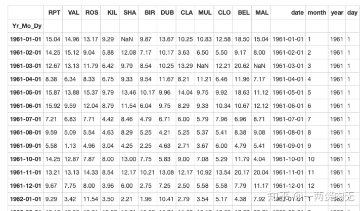
步骤13 对于数据记录按照月为频率取样

# 运行以下代码
data.query('day == 1')

out[303]:

练习7-可视化

探索泰坦尼克灾难数据

相应数据集：train.csv

步骤1 导入必要的库

# 运行以下代码
import pandas as pd
import matplotlib.pyplot as plt
import seaborn as sns
import numpy as np

%matplotlib inline

步骤2 从以下地址导入数据

# 运行以下代码
path7 = '../input/pandas_exercise/exercise_data/train.csv'  # train.csv

步骤3 将数据框命名为titanic

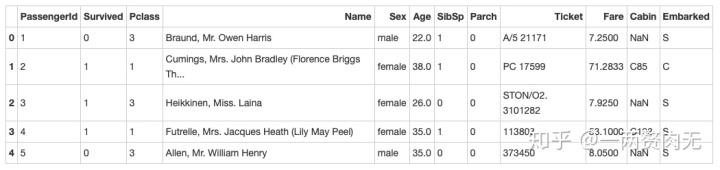
# 运行以下代码
titanic = pd.read_csv(path7)
titanic.head()

out[306]:

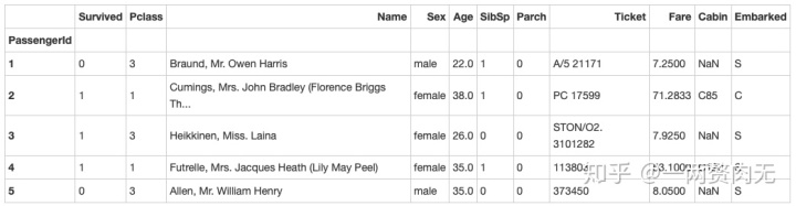
步骤4 将PassengerId设置为索引

# 运行以下代码
titanic.set_index('PassengerId').head()

out[307]:

步骤5 绘制一个展示男女乘客比例的扇形图

# 运行以下代码
# sum the instances of males and females
males = (titanic['Sex'] == 'male').sum()
females = (titanic['Sex'] == 'female').sum()

# put them into a list called proportions
proportions = [males, females]

# Create a pie chart
plt.pie(
    # using proportions
    proportions,
    
    # with the labels being officer names
    labels = ['Males', 'Females'],
    
    # with no shadows
    shadow = False,
    
    # with colors
    colors = ['blue','red'],
    
    # with one slide exploded out
    explode = (0.15 , 0),
    
    # with the start angle at 90%
    startangle = 90,
    
    # with the percent listed as a fraction
    autopct = '%1.1f%%'
    )

# View the plot drop above
plt.axis('equal')

# Set labels
plt.title("Sex Proportion")

# View the plot
plt.tight_layout()
plt.show()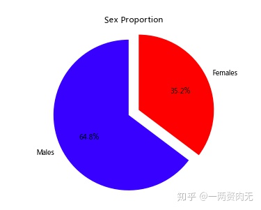

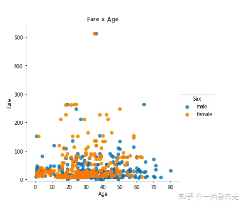
步骤6 绘制一个展示船票Fare, 与乘客年龄和性别的散点图

# 运行以下代码
# creates the plot using
lm = sns.lmplot(x = 'Age', y = 'Fare', data = titanic, hue = 'Sex', fit_reg=False)

# set title
lm.set(title = 'Fare x Age')

# get the axes object and tweak it
axes = lm.axes
axes[0,0].set_ylim(-5,)
axes[0,0].set_xlim(-5,85)

out[309]:

(-5, 85)

步骤7 有多少人生还？

# 运行以下代码
titanic.Survived.sum()

out[310]:

342

步骤8 绘制一个展示船票价格的直方图

# 运行以下代码
# sort the values from the top to the least value and slice the first 5 items
df = titanic.Fare.sort_values(ascending = False)
df

# create bins interval using numpy
binsVal = np.arange(0,600,10)
binsVal

# create the plot
plt.hist(df, bins = binsVal)

# Set the title and labels
plt.xlabel('Fare')
plt.ylabel('Frequency')
plt.title('Fare Payed Histrogram')

# show the plot
plt.show()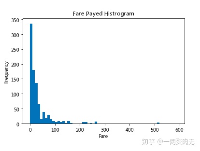

练习8-创建数据框

探索Pokemon数据

相应数据集：练习中手动内置的数据

步骤1 导入必要的库

# 运行以下代码
import pandas as pd

步骤2 创建一个数据字典

# 运行以下代码
raw_data = {"name": ['Bulbasaur', 'Charmander','Squirtle','Caterpie'],
            "evolution": ['Ivysaur','Charmeleon','Wartortle','Metapod'],
            "type": ['grass', 'fire', 'water', 'bug'],
            "hp": [45, 39, 44, 45],
            "pokedex": ['yes', 'no','yes','no']                        
            }

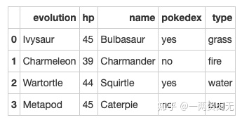
步骤3 将数据字典存为一个名叫pokemon的数据框中

# 运行以下代码
pokemon = pd.DataFrame(raw_data)
pokemon.head()

out[314]:

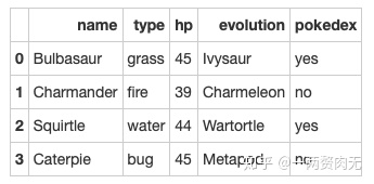
步骤4 数据框的列排序是字母顺序，请重新修改为name, type, hp, evolution, pokedex这个顺序

# 运行以下代码
pokemon = pokemon[['name', 'type', 'hp', 'evolution','pokedex']]
pokemon

out[315]:

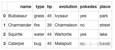
步骤5 添加一个列place

# 运行以下代码
pokemon['place'] = ['park','street','lake','forest']
pokemon 

out[316]:

步骤6 查看每个列的数据类型

# 运行以下代码
pokemon.dtypes

out[317]:
name object
type object
hp int64
evolution object
pokedex object
place object
dtype: object

练习9-时间序列

探索Apple公司股价数据

相应数据集：Apple_stock.csv

步骤1 导入必要的库

# 运行以下代码
import pandas as pd
import numpy as np

# visualization
import matplotlib.pyplot as plt

%matplotlib inline

步骤2 数据集地址

# 运行以下代码
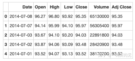
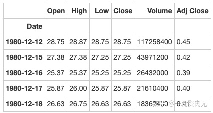
path9 = '../input/pandas_exercise/exercise_data/Apple_stock.csv'   # Apple_stock.csv

步骤3 读取数据并存为一个名叫apple的数据框

# 运行以下代码
apple = pd.read_csv(path9)
apple.head()

out[320]:

步骤4 查看每一列的数据类型

# 运行以下代码
apple.dtypes

out[321]:

Date object
Open float64
High float64
Low float64
Close float64
Volume int64
Adj Close float64
dtype: object

步骤5 将Date这个列转换为datetime类型

# 运行以下代码
apple.Date = pd.to_datetime(apple.Date)
apple['Date'].head()

out[322]:

0 2014-07-08
1 2014-07-07
2 2014-07-03
3 2014-07-02
4 2014-07-01
Name: Date, dtype: datetime64[ns]

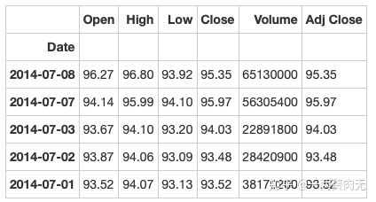
步骤6 将Date设置为索引

# 运行以下代码
apple = apple.set_index('Date')
apple.head()

out[323]:

步骤7 有重复的日期吗？

# 运行以下代码
apple.index.is_unique

out[324]:

True

步骤8 将index设置为升序

# 运行以下代码
apple.sort_index(ascending = True).head()

out[325]:

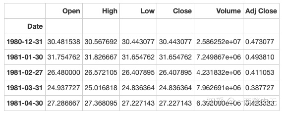
步骤9 找到每个月的最后一个交易日(business day)

# 运行以下代码
apple_month = apple.resample('BM')
apple_month.head()

out[326]:

步骤10 数据集中最早的日期和最晚的日期相差多少天？

# 运行以下代码
(apple.index.max() - apple.index.min()).days

out[327]:

12261

步骤11 在数据中一共有多少个月？

# 运行以下代码
apple_months = apple.resample('BM').mean()
len(apple_months.index)

out[328]:

404

步骤12 按照时间顺序可视化Adj Close值

# 运行以下代码
# makes the plot and assign it to a variable
appl_open = apple['Adj Close'].plot(title = "Apple Stock")

# changes the size of the graph
fig = appl_open.get_figure()
fig.set_size_inches(13.5, 9)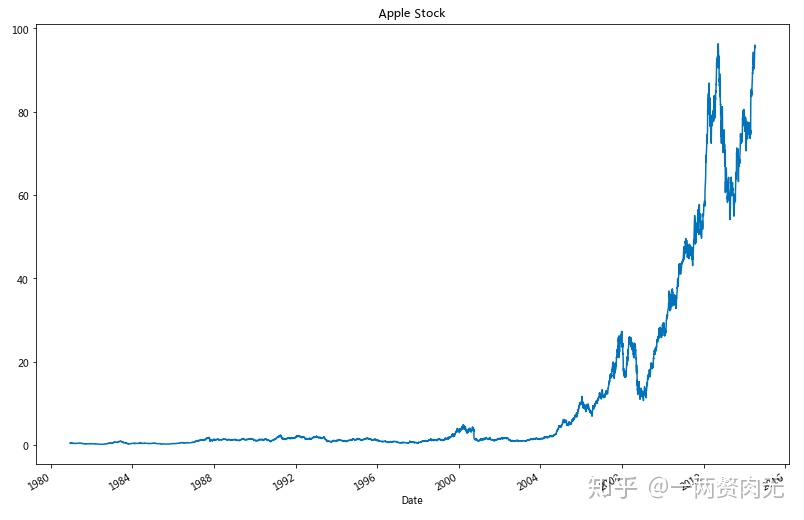

练习10-删除数据

探索Iris纸鸢花数据

相应数据集：iris.csv

步骤1 导入必要的库

# 运行以下代码
import pandas as pd

步骤2 数据集地址

# 运行以下代码
path10 ='../input/pandas_exercise/exercise_data/iris.csv'   # iris.csv

步骤3 将数据集存成变量iris

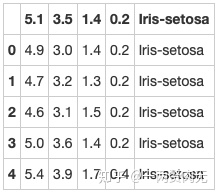
# 运行以下代码
iris = pd.read_csv(path10)
iris.head() 

out[332]:

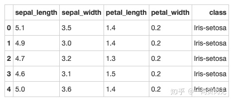
步骤4 创建数据框的列名称

iris = pd.read_csv(path10,names = ['sepal_length','sepal_width', 'petal_length', 'petal_width', 'class'])
iris.head()

out[333]:

步骤5 数据框中有缺失值吗？

# 运行以下代码
pd.isnull(iris).sum()

out[334]:

sepal_length 0
sepal_width 0
petal_length 0
petal_width 0
class 0
dtype: int64

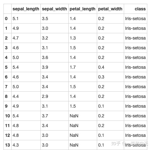
步骤6 将列petal_length的第10到19行设置为缺失值

# 运行以下代码
iris.iloc[10:20,2:3] = np.nan
iris.head(20)

out[335]:

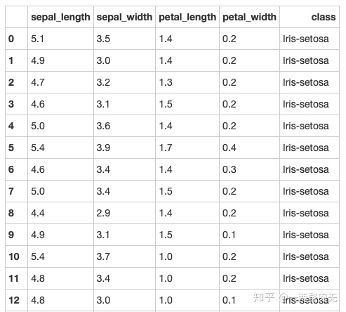
步骤7 将缺失值全部替换为1.0

# 运行以下代码
iris.petal_length.fillna(1, inplace = True)
iris

out[336]:

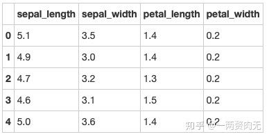
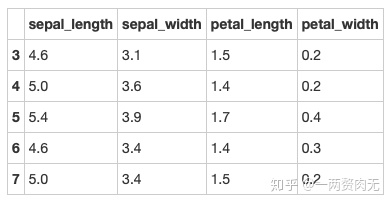
步骤8 删除列class

# 运行以下代码
del iris['class']
iris.head() 

out[337]:

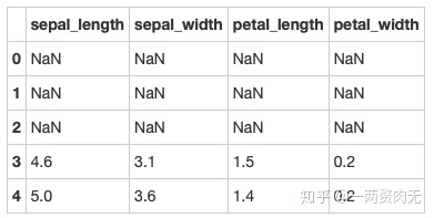
步骤9 将数据框前三行设置为缺失值

# 运行以下代码
iris.iloc[0:3 ,:] = np.nan
iris.head()

out[338]:

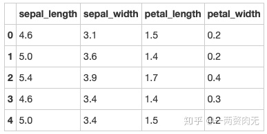
步骤10 删除有缺失值的行

# 运行以下代码
iris = iris.dropna(how='any')
iris.head()

out[339]:

步骤11 重新设置索引

# 运行以下代码
iris = iris.reset_index(drop = True)
iris.head()

out[340]:

转载本文请联系和鲸社区取得授权。