


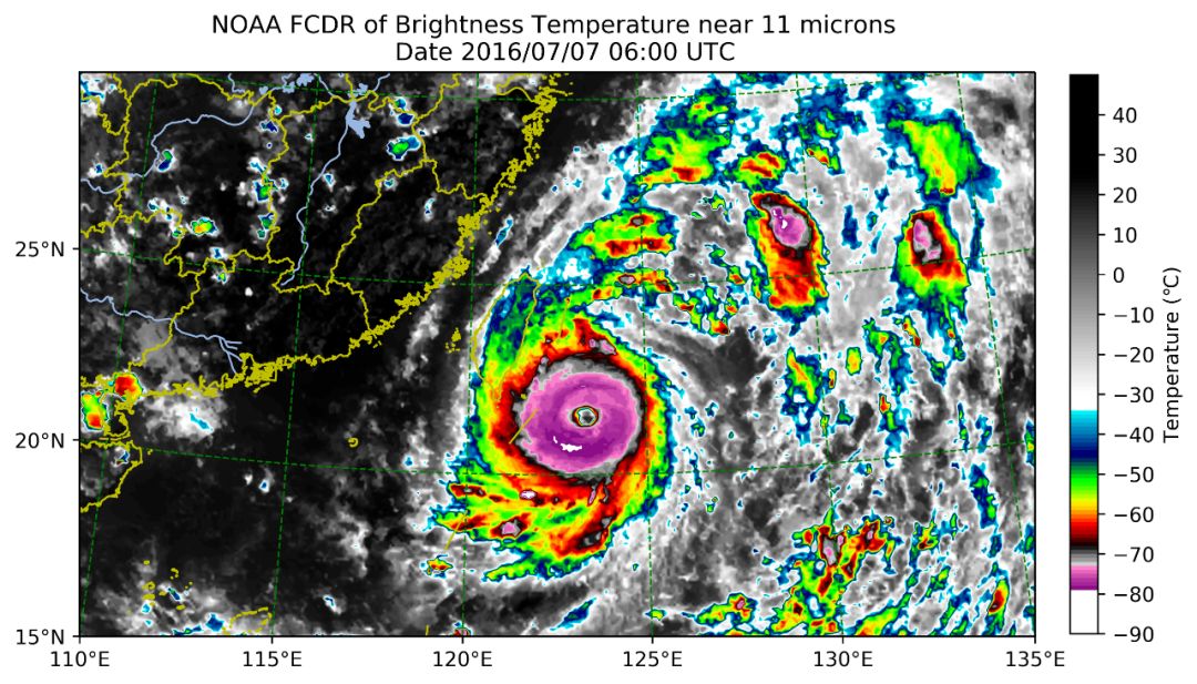
前段时间袭击中国的超强台风“利奇马”,以及这两天袭击美国的五级飓风“多利安”,让我们感受到了大自然的力量。所以,今天分享一个简单的Python实例,也算是延续前面python气象绘图系列(点击链接1;点击链接2),与大家交流如何选择合适的色标来绘制台风云顶亮温展示台风的部分特征。配色方案借鉴了GOES-16 Data[1]数据的处理方法。我们此次针对于中国区域进行一个展示,数据选取GridSat-B1 CDR(数据下载地址)[2]. A climate quality, long term dataset of global infrared window brightness temperatures. 1981-present (updated quarterly)。
如果在业务绘图或者科研中使用文中提供的脚本有问题,也欢迎加入MeteoAI的微信交流群一起交流,也可以添加我的微信(gavin7675)交流探讨。
对不起,放错图了!不过,动态展示台风也是很有必要,后续试着复现一下。

目标:绘制中国区域(邻近海域)台风,展示台风的部分特征,绘制经纬度网格线,附带经纬度信息,基本的地界信息。
工具:Python3.6+(Anaconda)、cpt文件/处理python脚本、地理界线、一系列相关的Python库、测试数据
1.出图
效果图:
2.数据、脚本
链接:https://pan.baidu.com/s/1lXA1jlmZrG09rj5OhAoSXg 密码:sojk
3.代码展示
import matplotlib
matplotlib.use('TkAgg')
import os,sys
import scipy.ndimage
import numpy as np
import xarray as xr
from copy import copy
import matplotlib.pyplot as plt # Import the Matplotlib package
from mpl_toolkits.basemap import Basemap # Import the Basemap toolkit
from cpt_convert import loadCPT # Import the CPT convert function
from matplotlib.colors import LinearSegmentedColormap # Linear interpolation for color maps
import cartopy.crs as ccrs
import cartopy.feature as cfeature
from cartopy.mpl.gridliner import LATITUDE_FORMATTER, LONGITUDE_FORMATTER
import shapely.geometry as sgeom

def find_side(ls, side):
    """
 Given a shapely LineString which is assumed to be rectangular, return the
 line corresponding to a given side of the rectangle.
 """
    minx, miny, maxx, maxy = ls.bounds
    points = {'left': [(minx, miny), (minx, maxy)],
              'right': [(maxx, miny), (maxx, maxy)],
              'bottom': [(minx, miny), (maxx, miny)],
              'top': [(minx, maxy), (maxx, maxy)],}
    return sgeom.LineString(points[side])

def lambert_xticks(ax, ticks):
    """Draw ticks on the bottom x-axis of a Lambert Conformal projection."""
    te = lambda xy: xy[0]
    lc = lambda t, n, b: np.vstack((np.zeros(n) + t, np.linspace(b[2], b[3], n))).T
    xticks, xticklabels = _lambert_ticks(ax, ticks, 'bottom', lc, te)
    ax.xaxis.tick_bottom()
    ax.set_xticks(xticks)
    ax.set_xticklabels([ax.xaxis.get_major_formatter()(xtick) for xtick in xticklabels])

def lambert_yticks(ax, ticks):
    """Draw ricks on the left y-axis of a Lamber Conformal projection."""
    te = lambda xy: xy[1]
    lc = lambda t, n, b: np.vstack((np.linspace(b[0], b[1], n), np.zeros(n) + t)).T
    yticks, yticklabels = _lambert_ticks(ax, ticks, 'left', lc, te)
    ax.yaxis.tick_left()
    ax.set_yticks(yticks)
    ax.set_yticklabels([ax.yaxis.get_major_formatter()(ytick) for ytick in yticklabels])

def _lambert_ticks(ax, ticks, tick_location, line_constructor, tick_extractor):
    """Get the tick locations and labels for an axis of a Lambert Conformal projection."""
    outline_patch = sgeom.LineString(ax.outline_patch.get_path().vertices.tolist())
    axis = find_side(outline_patch, tick_location)
    n_steps = 30
    extent = ax.get_extent(ccrs.PlateCarree())
    _ticks = []
    for t in ticks:
        xy = line_constructor(t, n_steps, extent)
        proj_xyz = ax.projection.transform_points(ccrs.Geodetic(), xy[:, 0], xy[:, 1])
        xyt = proj_xyz[..., :2]
        ls = sgeom.LineString(xyt.tolist())
        locs = axis.intersection(ls)
        if not locs:
            tick = [None]
        else:
            tick = tick_extractor(locs.xy)
        _ticks.append(tick[0])
    # Remove ticks that aren't visible:
    ticklabels = copy(ticks)
    while True:
        try:
            index = _ticks.index(None)
        except ValueError:
            break
        _ticks.pop(index)
        ticklabels.pop(index)
    return _ticks, ticklabels


# 区域选择
lat_s = 15
lat_n = 30
lon_w = 110
lon_e = 135


# Load the border data, CN-border-La.dat is downloaded from
# https://gmt-china.org/data/CN-border-La.dat
with open('CN-border-La.dat') as src:
    context = src.read()
    blocks = [cnt for cnt in context.split('>') if len(cnt) > 0]
    borders = [np.fromstring(block, dtype=float, sep=' ') for block in blocks]


path = '/Users/zhpfu/Dropbox/Code_Fortress/00_My_Python_Library/Typhoon/GRIDSAT-B1.2016.07.07.06.v02r01.nc'

# Search for the Scan start in the file name  2016.07.07.06
Start = (path[path.find("B1.")+3:path.find(".v02")])
Start_Formatted = " Date "+ Start[0:4] + "/" + Start[5:7] + "/" + Start [8:10]+ " " + Start [11:13]+":00 UTC"

print(Start_Formatted)


# Set figure size
proj = ccrs.LambertConformal(central_longitude=(lon_w+lon_e)/2., central_latitude= (lat_s+lat_n)/2.,
                             false_easting=400000, false_northing=400000)#,standard_parallels=(46, 49))

fig = plt.figure(figsize=[10, 8],frameon=True)

print("AAAAAA")

# Set projection and plot the main figure
ax = fig.add_axes([0.08, 0.05, 0.8, 0.94], projection=proj)

# Set figure extent
ax.set_extent([lon_w, lon_e, lat_s, lat_n],crs=ccrs.PlateCarree())

# Plot border lines
for line in borders:
    ax.plot(line[0::2], line[1::2], '-', lw=1.0, color='y',
            transform=ccrs.Geodetic())

# Add ocean, land, rivers and lakes
ax.add_feature(cfeature.OCEAN.with_scale('50m'))
ax.add_feature(cfeature.LAND.with_scale('50m'))
ax.add_feature(cfeature.RIVERS.with_scale('50m'))
ax.add_feature(cfeature.LAKES.with_scale('50m'))

print("BBBBBB")

# *must* call draw in order to get the axis boundary used to add ticks:
fig.canvas.draw()

# Define gridline locations and draw the lines using cartopy's built-in gridliner:
# xticks = [] ; yticks = []
npts   = 5
xticks = list(np.arange(lon_w-15,lon_e+15+1,npts))
yticks = list(np.arange(lat_s-15,lat_n+15+1,npts))


ax.gridlines(xlocs=xticks, ylocs=yticks,linestyle='--',lw=0.85,color='green')# dimgrey

# Label the end-points of the gridlines using the custom tick makers:
ax.xaxis.set_major_formatter(LONGITUDE_FORMATTER)
ax.yaxis.set_major_formatter(LATITUDE_FORMATTER)

# https://stackoverflow.com/questions/30030328/correct-placement-of-colorbar-relative-to-geo-axes-cartopy
lambert_xticks(ax, xticks)
lambert_yticks(ax, yticks)


print("CCCCCC")

# Converts a CPT file to be used in Python
cpt = loadCPT('IR4AVHRR6.cpt')
# Makes a linear interpolation
cpt_convert = LinearSegmentedColormap('cpt', cpt)


ds    = xr.open_dataset(path)
lat   = ds.lat
lon   = ds.lon
time  = ds.time
data0 = (ds['irwin_cdr'][0,:,:] - 273.15 ) # 把温度转换为℃  - 273.15


lon_range = lon[(lon>lon_w-5) & (lon5)]
lat_range = lat[(lat>lat_s-5) & (lat5)]
data     = data0.sel(lon=lon_range, lat=lat_range)
print(data)
print(time)# 设置colorbar #get size and extent of axes:
cbar_kwargs = {'orientation': 'vertical',    #'horizontal','label': 'Temperature (℃)','ticks': np.arange(-90, 40 + 1, 10),'pad': 0.03,'shrink': 0.51
}
levels = np.arange(-90, 50 + 1, 1) # .reversed() ,, vmin=-90, vmax=50, .reversed() # # Resample your data grid by a factor of 3 using cubic spline interpolation.# data = scipy.ndimage.zoom(data, 3)# # from scipy.ndimage.filters import gaussian_filter# sigma = 0.7 # this depends on how noisy your data is, play with it!# data = gaussian_filter(data, sigma)#
data.plot.contourf(ax=ax, levels=levels, vmin=-90, vmax=50, cmap=cpt_convert, origin='upper',
                   cbar_kwargs=cbar_kwargs, transform=ccrs.PlateCarree())#http://xarray.pydata.org/en/stable/plotting.html
plt.ylabel('')    #Remove the defult  lat / lon label
plt.xlabel('')
print("DDDDDD")# Add a title to the plot
plt.title("NOAA FCDR of Brightness Temperature near 11 microns "+ "\n " + Start_Formatted)# Save & Show figure
(filename, extension) = os.path.splitext(os.path.basename(sys.argv[0]))
plt.savefig(filename+".png", dpi=600, bbox_inches='tight')
print("EEEEEE")
plt.show()本文同步更新在微信公众号『气象学家』
往期推荐
Pandas从小白到大师 Python绘制气象实用地图[Code+Data](续) Python绘制气象实用地图(附代码和测试数据) 用机器学习应对气候变化? 最易写出bug?Python命名空间和作用域介绍 捍卫祖国领土从每一张地图开始 Nature(2019)-地球系统科学领域的深度学习及其理解 交叉新趋势|采用神经网络与深度学习来预报降水、温度等案例(附代码/数据/文献)References
[1] GOES-16 Data: https://geonetcast.wordpress.com/2017/06/02/geonetclass-manipulating-goes-16-data-with-python-part-v/[2] (数据下载地址): https://www.ncdc.noaa.gov/gridsat/gridsat-index.php


 被折叠的 条评论
为什么被折叠?
被折叠的 条评论
为什么被折叠?
 到【灌水乐园】发言


