python onehot编码_使用Python线性回归预测Steam游戏的打折的幅度

上篇文章我们解决了Steam是否打折的问题，这篇文章我们要解决的是到底打折幅度有多少，这里我们就不能使用分类模型，而需要使用回归的模型了。

主要目标

在这个项目中，我将试图找出什么样的因素会影响Steam的折扣率并建立一个线性回归模型来预测折扣率。

数据

数据将直接从Steam的官方网站上获取。

我们使用Python编写抓取程序，使用的库包括：

"re"— regex"，用于模式查找。

"CSV"— 用于将刮下的数据写入.CSV文件中，使用pandas进行处理。

"requests"— 向Steam网站发送http/https请求

"BeautifulSoup"—用于查找html元素/标记。

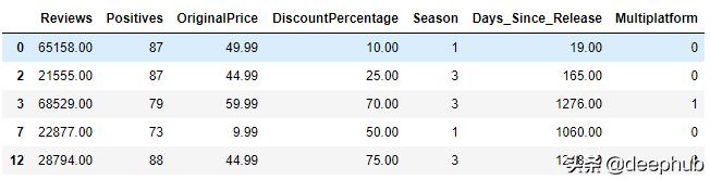
当数据加载到Pandas中时，大概的显示如下所示：

我们训练模型的目标是:数据集中预测的目标是"折扣百分比",DiscountPercentage

数据清洗

采集的原始数据包含许多我们不需要的东西：

一、 免费游戏，没有价格，包括演示和即将发布。

二、不打折的游戏。

三、非数值的数据

我们在把他们清洗的同时，还可以做一些特征工程。

在后面的章节中，我将介绍在建模和测试时所做的所有特性工程，但是对于基线模型，可以使用以下方式

添加一个"季节"栏，查看游戏发布的季节：

完成上述过程后，我们现在可以从dataframe中删除所有基于字符串的列：

这个过程还将把我们的结果从14806个和12个特征缩小到370个条目和7个特征。

不好的消息是这意味着由于样本量较小，该模型很容易出现误差。

数据分析

分析部分包括三个步骤：

1. 数据探索分析(EDA)

1. 特征工程(FE)

1. 建模

一般工作流程如下所示：

EDA以找到的特征-目标关系(通过对图/热图、Lasso 系数等)

根据可用信息，进行特征工程(数学转换、装箱、获取虚拟条目

使用R方和/或其他指标(RMSE、MAE等)建模和评分

冲洗并重复以上步骤，直到尝试并用尽所有潜在的特征工程想法或达到可接受的评分分数(例如R方)。

# Plotting heat map as part of EDAsns.heatmap(df.corr(),cmap="YlGnBu",annot=True)plt.show()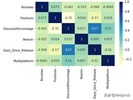

# A compiled function to automatically split data, make and score models. And showing you what's the most relevant features.def RSquare(df, col):    X, y = df.drop(col,axis=1), df[col]    X, X_test, y, y_test = train_test_split(X, y, test_size=.2, random_state=10) #hold out 20% of the data for final testing    #this helps with the way kf will generate indices below    X, y = np.array(X), np.array(y)        kf = KFold(n_splits=5, shuffle=True, random_state = 50)    cv_lm_r2s, cv_lm_reg_r2s, cv_lm_poly_r2s, cv_lasso_r2s = [], [], [], [] #collect the validation results for both models    for train_ind, val_ind in kf.split(X,y):        X_train, y_train = X[train_ind], y[train_ind]        X_val, y_val = X[val_ind], y[val_ind]         #simple linear regression        lm = LinearRegression()        lm_reg = Ridge(alpha=1)        lm_poly = LinearRegression()        lm.fit(X_train, y_train)        cv_lm_r2s.append(lm.score(X_val, y_val))        #ridge with feature scaling        scaler = StandardScaler()        X_train_scaled = scaler.fit_transform(X_train)        X_val_scaled = scaler.transform(X_val)        lm_reg.fit(X_train_scaled, y_train)        cv_lm_reg_r2s.append(lm_reg.score(X_val_scaled, y_val))        poly = PolynomialFeatures(degree=2)         X_train_poly = poly.fit_transform(X_train)        X_val_poly = poly.fit_transform(X_val)        lm_poly.fit(X_train_poly, y_train)        cv_lm_poly_r2s.append(lm_poly.score(X_val_poly, y_val))                #Lasso        std = StandardScaler()        std.fit(X_train)                X_tr = std.transform(X_train)        X_te = std.transform(X_test)                X_val_lasso = std.transform(X_val)                alphavec = 10**np.linspace(-10,10,1000)        lasso_model = LassoCV(alphas = alphavec, cv=5)        lasso_model.fit(X_tr, y_train)        cv_lasso_r2s.append(lasso_model.score(X_val_lasso, y_val))                test_set_pred = lasso_model.predict(X_te)                column = df.drop(col,axis=1)        to_print = list(zip(column.columns, lasso_model.coef_))        pp = pprint.PrettyPrinter(indent = 1)            rms = sqrt(mean_squared_error(y_test, test_set_pred))            print('Simple regression scores: ', cv_lm_r2s, '')    print('Ridge scores: ', cv_lm_reg_r2s, '')    print('Poly scores: ', cv_lm_poly_r2s, '')    print('Lasso scores: ', cv_lasso_r2s, '')    print(f'Simple mean cv r^2: {np.mean(cv_lm_r2s):.3f} +- {np.std(cv_lm_r2s):.3f}')    print(f'Ridge mean cv r^2: {np.mean(cv_lm_reg_r2s):.3f} +- {np.std(cv_lm_reg_r2s):.3f}')    print(f'Poly mean cv r^2: {np.mean(cv_lm_poly_r2s):.3f} +- {np.std(cv_lm_poly_r2s):.3f}', '')        print('lasso_model.alpha_:', lasso_model.alpha_)    print(f'Lasso cv r^2: {r2_score(y_test, test_set_pred):.3f} +- {np.std(cv_lasso_r2s):.3f}', '')        print(f'MAE: {np.mean(np.abs(y_pred - y_true)) }', '')    print('RMSE:', rms, '')        print('Lasso Coef:')    pp.pprint (to_print)

先贴一些代码，后面做详细解释

第一次尝试：基本模型,删除评论少于30条的游戏

# Setting a floor limit of 30df1 = df1[df1.Reviews > 30]

Best Model: LassoScore: 0.419 +- 0.073

第二次："Reviews" & "OriginalPrice" 进行对数变换

df2.Reviews = np.log(df2.Reviews)df2.OriginalPrice = df2.OriginalPrice.astype(float)df2.OriginalPrice = np.log(df2.OriginalPrice)

Best Model: Lasso Score: 0.437 +- 0.104

第三次：将mantag进行onehot编码

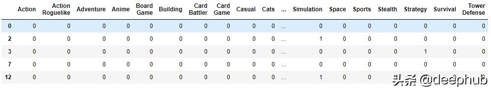
# Checking to make sure the dummies are separated correctlypd.get_dummies(df3.Main_Tag).head(5)# Adding dummy categories into the dataframedf3 = pd.concat([df3, pd.get_dummies(df3.Main_Tag).astype(int)], axis = 1)# Drop original string based column to avoid conflict in linear regressiondf3.drop('Main_Tag', axis = 1, inplace=True)

Best Model: Lasso Score: 0.330 +- 0.073

第四次：尝试把所有非数值数据都进行onehot编码

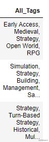
# we can get dummies for each tag listed separated by commasplit_tag = df4.All_Tags.astype(str).str.strip('[]').str.get_dummies(', ')# Now merge the dummies into the data frame to start EDAdf4= pd.concat([df4, split_tag], axis=1)# Remove any column that only has value of 0 as precautiondf4 = df4.loc[:, (df4 != 0).any(axis=0)]

Best Model: Lasso Score: 0.359 +- 0.080

第五次：整合2和4次操作

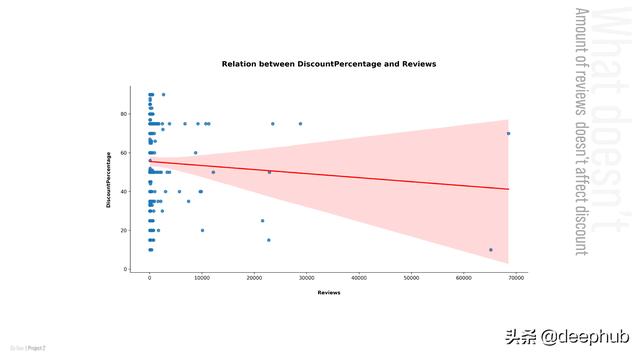
# Dummy all top 5 tagssplit_tag = df.All_Tags.astype(str).str.strip('[]').str.get_dummies(', ')df5= pd.concat([df5, split_tag], axis=1)# Log transform Review due to skewed pairplot graphsdf5['Log_Review'] = np.log(df5['Reviews'])

Best Model: Lasso Score: 0.359 +- 0.080

看到结果后，发现与第4次得分完全相同，这意味着"评论"对折扣百分比绝对没有影响。所以这一步操作可以不做，对结果没有任何影响

第六次：对将"评论"和"发布后的天数"进行特殊处理

# Binning reviews (which is highly correlated with popularity) based on the above 75 percentile and 25 percentiledf6.loc[df6['Reviews'] < 33, 'low_pop'] = 1df6.loc[(df6.Reviews >= 33) & (df6.Reviews < 381), 'mid_pop'] = 1df6.loc[df6['Reviews'] >= 381, 'high_pop'] = 1# Binning Days_Since_Release based on the above 75 percentile and 25 percentiledf6.loc[df6['Days_Since_Release'] < 418, 'new_game'] = 1df6.loc[(df6.Days_Since_Release >= 418) & (df6.Days_Since_Release < 1716), 'established_game'] = 1df6.loc[df6['Days_Since_Release'] >= 1716, 'old_game'] = 1# Fill all the NaN'sdf6.fillna(0, inplace = True)# Drop the old columns to avoid multicolinearitydf6.drop(['Reviews', 'Days_Since_Release'], axis=1, inplace = True)

这两列被分成三个特征。

Best Model: Ridge Score: 0.273 +- 0.044

第七次：拆分其他特征并删除不到30条评论的结果。

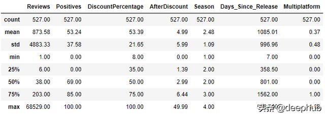
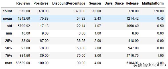
# Setting a floor threshold of 30 reivews for the data frame to remove some outliersdf7 = df7[df7.Reviews > 30]# Binning based on 50%df7.loc[df7['Reviews'] < 271, 'low_pop'] = 1df7.loc[df7['Reviews'] >= 271, 'high_pop'] = 1df7.loc[df7['Days_Since_Release'] < 1167, 'new_game'] = 1df7.loc[df7['Days_Since_Release'] >= 1167, 'old_game'] = 1# Fill all NaN'sdf7.fillna(0, inplace= True)# Drop old columns to avoid multicolinearitydf7.drop(['Reviews', 'Days_Since_Release'], axis=1, inplace = True)

Best Model: Lasso Score: 0.313 +- 0.098

清洗总结：让我们从数据清理产生的一些统计数据开始：

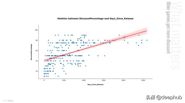
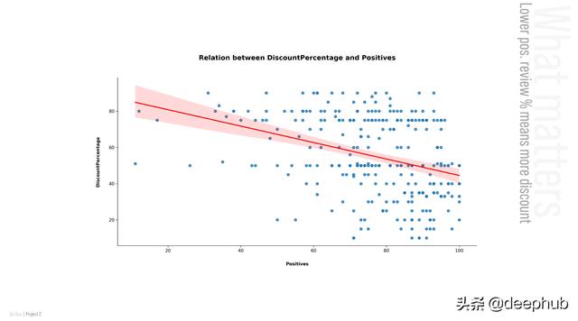
现在，让我们看看影响折扣率的前两个特性是什么：

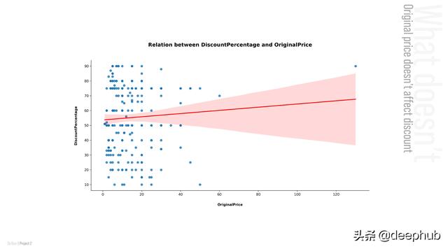
但是什么不影响折扣率呢？让我们看看不影响折扣率的前两个特性是什么：

最好的模型实际上是误差最小的基线模型。

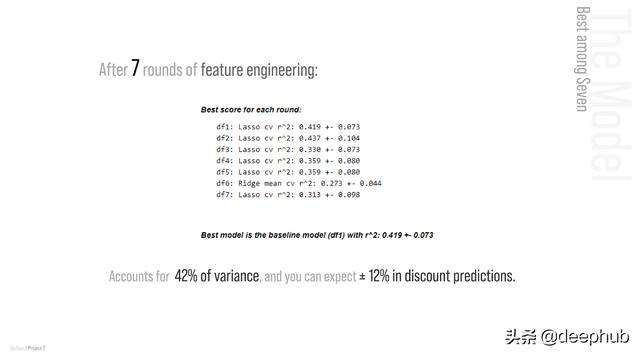
0.42的R方看起来并不是很好，但是这与Steam如何处理折扣有很大关系-因为只有出版商/开发商才有权对他们的游戏进行打折。

这意味着折扣率将在很大程度上取决于每个出版商/开发商的营销策略和他们的财务状况。虽然我希望将来情况会有所改善，但我目前无法收集到这样的数据。

用户案例

这个模型看起来好像没什么实际用处，其实它也有实际的意义——它对在线视频游戏转售商来说将特别有用。

如上图所示，我的预测模型可以帮助他们预测下一个大折扣，这样他们就可以更好地分配资源，潜在地增加利润率。

本文作者：Da Guo

github项目地址：https://github.com/opophehu/LR_Steam