


The central experimental result of this work is an observation of distinct temperature and magnetic field dependences of the 7Li NMR relaxation rate \({T}_{1}^{-1}\) in the short-range ordered (SRO) state of LiCuSbO4 below ~10 K, as shown in Fig. 5, which will be discussed in the following.
NMR relaxation in magnetic solids
In magnetic materials, the nuclear spin lattice relaxation rate, \({T}_{1}^{-1}\), is typically caused by the transverse (i.e. ⊥ to the nuclear spin quantization axis) components of the time-dependent fluctuating field exerted on the nuclei by the electron spin system. It can be expressed in terms of the Fourier transforms \({S}^{z,\pm }(q,\omega )\) of the time-dependent longitudinal and transverse spin-spin correlation functions \(\langle {S}_{j}^{z}(t){S}_{0}^{z}\mathrm{(0)}\rangle \), \(\langle {S}_{j}^{+}(t){S}_{0}^{-}\mathrm{(0)}\rangle \) and \(\langle {S}_{j}^{-}(t){S}_{0}^{+}\mathrm{(0)}\rangle \), respectively
$$\begin{array}{rcl}{S}^{z,\pm }(q,\omega ) & = & \sum _{j}\,{e}^{-iqj}{\int }_{-\infty }^{\infty }\,dt{e}^{i\omega t}{\langle {S}_{j}^{z,\pm }(t){S}_{0}^{z,\mp }\mathrm{(0)}\rangle }_{T},\\ \quad \quad \,\,\,{T}_{1}^{-1} & \propto & \frac{{\gamma }_{n}^{2}}{{\gamma }_{e}^{2}}\mathop{\mathrm{lim}}\limits_{\omega \to 0}\sum _{q}\,{|{A}_{\parallel }(q)|}^{2}{S}^{z}(q,\omega )\\ & & +{|{A}_{\perp }(q)|}^{2}[{S}^{\pm }(q,\omega )+{S}^{\mp }(q,\omega )].\end{array}$$
(1)
Here q is the wave vector, \({\langle \cdots \rangle }_{T}\) means the thermal average, γ
e/n are the gyromagnetic ratios of the electron and the probed nucleus, and \({A}_{\parallel ,\perp }(\overrightarrow{q})\) are the hyperfine form factors of the probed nucleus. The subscripts \(\parallel \) and \(\perp \) denote the hyperfine tensor components generating the transversal components of the fluctuating local field at the nuclear site due to the longitudinal 〈zz〉 and transversal 〈+ −〉 spin-spin correlations, respectively. For \(\hslash {\omega }_{{\rm{NMR}}}\ll {k}_{{\rm{B}}}T\), \({S}^{z,\pm }(q,\omega )\propto {\chi }_{z,\pm }^{^{\prime\prime} }(q,\omega ){k}_{{\rm{B}}}T/\hslash {\omega }_{{\rm{NMR}}}\), where \({\chi }_{z,\pm }^{^{\prime\prime} }(q,\omega )\) is the imaginary part of the dynamical electron spin susceptibility, \({\omega }_{{\rm{NMR}}}\) is the NMR frequency, k
B and ħ are the Boltzmann’s constant and the reduced Planck constant, respectively. Thus at small NMR frequencies, \(1/{T}_{1}\propto {\sum }_{q}\,\chi ^{\prime\prime} (q,\omega \to 0)T\).
Generally, filtering effects may occur such that the hyperfine coupling is peaked (or zero) for certain q-vectors. However, the crystal structure of LiCuSbO4 indicates that both Li sites are coupled to several Cu sites from different chains, suggesting a rather weak dependence of \({A}_{\parallel ,\perp }\) on q. Since the coupling between the 7Li nuclear spin and the Cu spins is of dipolar nature both the longitudinal and the transversal terms in Eq. (1) are expected to contribute to the relaxation. Indeed, our estimates with the dipolar hyperfine model have revealed comparable contributions from 〈zz〉 and 〈+ −〉 correlations to the transversal field at both Li sites (see, Suppl.).
Field dependence of T1
−1
In weakly coupled unfrustrated critical simple AFM Heisenberg chains in the paramagnetic state far above the Neél ordering temperature \({T}_{{\rm{N}}}\ll T\ll J/{k}_{{\rm{B}}}\), the rate \({T}_{1}^{-1}\) in general continuously increases with decreasing T and/or increasing the magnetic field H up to the saturation field and tends to diverge by approaching T
N. This is mainly due to the growth of the \(\langle {S}_{j}^{+}(t){S}_{0}^{-}\mathrm{(0)}\rangle \) correlation function with increasing H and decreasing T whereas \(\langle {S}_{j}^{z}(t){S}_{0}^{z}\mathrm{(0)}\rangle \) decays smoothly following a power law
In LiCuSbO4, however, \({T}_{1}^{-1}\) shows a non-monotonous and even contrasting behavior with respect to temperature and magnetic field. At relatively small fields the low-temperature region is determined by a more or less sharp increase of \({T}_{1}^{-1}\) (T) (Fig. 5) pointing to the vicinity of a critical magnetically ordered state at a lower temperature. Especially at μ
0 H = 9 T the increase is substantially more pronounced than at lower fields such as for 3 T indicating an increase of the ordering temperature of the presumable magnetic phase. Such a behavior is not expected for an ordinary antiferromagnetic Neél state where T
N is usually suppressed by an external magnetic field. In fact, the field region around 9 T is also identified by the low-temperature anomaly in the magnetic specific heat in ref. 26. It has been conjectured in that work to be a signature of an unusual field-induced magnetic phase in LiCuSbO4.
One further and even more striking feature, which can be easily recognized in Fig. 5, is the occurrence of a threshold field of ~13 T that separates the upturn behavior from a drastic suppression of \({T}_{1}^{-1}\) vs. T. Indeed, plotting these data points for fixed temperatures as a function of the field, yields a set of curves with a sharp general crossing point at \({\mu }_{0}{H}_{{\rm{c}}1}\approx 13\,{\rm{T}}\), usually denoted in the literature as an isosbestic point (IBP)6). Since the nuclear \({T}_{1}^{-1}\) is governed by fluctuating fields at the nuclear site produced by electron spins, the IBP at 13 T may be identified as the critical field that separates two regimes with different types of magnetic fluctuations to be discussed in detail below. Indeed, at low-temperatures T ≤ 10–15 K which are of special interest here, the observed IBP coincides also with an inflection point (IFP). Using the generic linear field dependence \(1/{T}_{1}-const\propto (H-{H}_{{\rm{c}}1})\) in the vicinity of an IFP at H
c1, it is tempting to generalize that linear behavior further into the nonlinear region at higher fields employing a quasi-exponential expression that captures also the field region slightly smaller than H
c1:
$${T}_{1}^{-1}(H)=\frac{1}{{T}_{1}\,({H}_{{\rm{c}}1})}\,[1+0.92\,\tanh \,\frac{H-{H}_{{\rm{c}}1}}{1.12A}].$$
(2)
Here \(1/{T}_{1}({\mu }_{0}{H}_{{\rm{c}}1}=13\,{\rm{T}})=110\,{{\rm{s}}}^{-1}\) and A is a dimensional constant taken as 1 T. As can be seen in Fig. 6, Eq. (2) describes the data in the considered field region for the lowest available temperature T = 2.2 K quite well. This way we arrive at a smooth transition across H
c1 to a pronounced exponential-type behavior at high magnetic fields and low temperature.
Figure 6

The extracted spin-lattice relaxation rate 1/T
1 vs. external magnetic field for selected temperatures. Full lines are guides for the eye. The isosbestic point (IBP) near ~13 T is indicated by the vertical dashed line. The dashed orange curve is the fit to Eq. (2). (see the text).
Temperature dependence of T1
−1
Importantly, as can be seen in a logarithmic plot of \({T}_{1}^{-1}\) vs. T
−1 in Fig. 5(c,d), a similar predominantly exponential behavior develops for the strongest fields also in the T-dependence of \({T}_{1}^{-1}\) suggesting the opening of an energy gap for spin excitations. For a consistent analysis of the whole set of experimental \({T}_{1}^{-1}\) (T) curves we have used a phenomenological combined gapped and power-law ansatz which takes into account theoretical predictions in refs 36 and 37 (see discussion below):
$${T}_{1}^{-1}(T)={C}_{1}(H)\,\exp \,(-{\rm{\Delta }}/T)+{C}_{2}(H)\,{(T-{T}_{c})}^{\beta }.$$
(3)
Here, C
1 and C
2 are the weighting factors of the two contributions, Δ is the gap, and T
c and β are the critical temperature and the exponent of the power-law contribution, respectively. Possible T-dependences of the prefactors C
i remain unknown so far and have been not considered here. Though polycrystallinity of the samples and a certain distribution of the relaxation rates at highest fields and lowest temperatures (Suppl., Fig. S2) are complicating factors for the analysis, the \({T}_{1}^{-1}\) (T) dependences for all applied fields can be consistently modelled yielding a good description of the experimental data as shown in Fig. 5. The field dependences of the parameters of Eq. (3) are plotted in the Suppl., Fig. S3. The critical power-law behavior of \({T}_{1}^{-1}\) (T) at 3 T which sets in at \(T\mathop{ < }\limits_{ \tilde {}}7\,{\rm{K}}\) is fully consistent with the growth of the short-ranged incommensurate correlations reported for this temperature regime in ref. 26. The fit requires a very small T
c ~ 0.2 K suggesting that the 3D long-range magnetic order, if present at all, is shifted to very low temperatures. At 9 T, however, T
c is pushed up to ~1.5 K indicating the proximity to a new, field-induced magnetic state that has been revealed in the specific heat data in ref. 26. Further increase of the field up to 12 T yields a reduction of T
c down to ~1 K, again consistent with the fading of the magnetic anomaly in the specific heatH = 12 T requires a non-zero gap value Δ ~ 2 K in the first term of Eq. (3) implying the contrasting gapped and critical power-law contributions to \({T}_{1}^{-1}\) (T) with Δ > 0 and β
1 of the gapped term in Eq. (3) increases on expense of the decreasing weight C
2 of the power-law term (Suppl., Fig. S3). At the same time Δ increases non-linearly (Fig. 7). Despite the smallness of the weighting factor C
2 at H > H
c1, the finite power law contribution T
β in Eq. (3) with positive β, in contrast to β
c1, is required to achieve the best fit of \({T}_{1}^{-1}\) (T).
Figure 7

Magnetic field dependence of the gap Δ (squares) evaluated using Eq. (3). Dashed line connecting the data points is guide for the eye. Dotted line is a linear fit revealing the slope Δ/H = 1.56 K/T; Inset: the same for the exponent β in Eq. (3) (circles). Vertical dashed lines denote the isosbestic point H
c1 ≈ 13 T. Shaded bar indicates a crossover region between the two distinct regimes of the 7Li T
1 relaxation. (see the text).
Exclusion of an ordinary spin gap
In principle, there is a variety of conventional reasons for the opening of a gap in the spin excitation spectrum of a quantum magnet exposed to an external field. Generally, above saturation where the spins are fully polarized, all excitations acquire a gap that linearly scales with H. In the frustrated J
1(FM) − J
2(AFM) chain a two-magnon excitation is expected to have the lowest energy (see, e.g., ref. 16). In the case of LiCuSbO4, neglecting the non-linearity of the Δ(H) dependence in the crossover region, the increase of Δ amounts to Δ/μ0
H = 1.56 K/T (Fig. 7). This slope is in accord with the Zeeman energy of the flip of a single spin, i.e. a one-magnon excitation, which with the g-factor g = 2.18 obtained in the ESR experiment would amount to gμ
B/μ
0
k
B = 1.47 K/T. Correspondingly, the two-magnon slope should be ~3 K/T. Anyhow, we note that it would be unreasonable to identify \({\mu }_{0}{H}_{{\rm{c}}1}\approx 13\,{\rm{T}}\) as an effective saturation field. Our measurements of the static magnetization at very low T did not reveal a saturation of M(H) even in 20 T [Fig. 3(a)]. This finding is supported by our DMRG results (see below) showing that in a situation of the symmetric exchange anisotropy present in LiCuSbO4, there is no well defined saturation field at all in a literal sense, i.e. the full saturation at T = 0 is achieved only asymptotically [Fig. 8(a)].
Figure 8

(a) Experimental magnetization curve at 0.45 K and theoretical magnetization curve calculated for \(({J}_{1}^{x},{J}_{1}^{y},{J}_{1}^{z})=(-1.07,-0.99,-1)\) and J
2 = 0.28. Inset: enlarged figure around kink in the theoretical curve. (b) Nematic correlation for a homogeneous DM coupling γ = 0, 0.02, 0.04, and 0.06. (c) The same for a staggered DM coupling. (d) Temperature dependence of the nematic correlation. The shaded area depicts the field range where a spin gap was observed in the NMR experiment.
Another possible reason for a field induced gap could be the presence of staggered antisymmetric Dzyaloshinskii-Moriya (DM) interactions. Due to the low crystallographic symmetry, various DM interactions are generally allowed in LiCuSbO4 (see below). Their magnitude in LiCuSbO4 can be judged from the ESR data, because ESR is very sensitive to magnetic anisotropies. Assuming that the strongest antisymmetric DM coupling is present for the intra-chain NN bond with the DM vectors perpendicular to the Cu chain (see Fig. 1 and Suppl.), a strongly anisotropic gap should open for fields applied along the chainH
3 at low temperatures \(T < J/{k}_{{\rm{B}}}\)
3(c)] which suggests that the staggered DM component of the antisymmetric exchange is small in LiCuSbO4. The uniform component of the DM exchange can give rise to a field independent anisotropic gap which for certain field orientations may yield a splitting of the ESR signal4 is indeed found at high fields [Fig. 3(c)]. Its extend of the order ≈±30 GHz = ±1.5 K could give then the energy scale of the uniform DM component which is of a percent order of the isotropic and symmetric anisotropic exchange couplings as estimated from the magnetization data (see below).
Evidence for spin-nematicity
Ruling out the above discussed ordinary grounds for the field-dependent spin gap in LiCuSbO4 enables us now to focus on a possible, more sophisticated reason for the gap opening by approaching the IBP \({\mu }_{0}{H}_{{\rm{c}}1}\approx 13\,{\rm{T}}\) from the low-field side. According to the proposed theoretical precursor phase diagram of the isotropic frustrated J
1 − J
2 spin chainp = 2), corresponding to a precursor of a quadrupolar (spin-nematic) phase with a finite four-spin correlation function \(\langle {S}_{j}^{+}{S}_{j+1}^{+}{S}_{0}^{-}{S}_{1}^{-}\rangle \) is the simplest one. At the lower side of this field region a collinear and incommensurate quasi long-range ordered SDW2-phase is stabilized since \(\langle {S}_{j}^{z}{S}_{0}^{z}\rangle \) is the slowest decaying correlator. At the higher field side, above a certain crossover field, the quadrupolar 〈+ + − −〉 correlations might become nevertheless dominant yielding a competing quasi long-range ordered pronounced spin-nematic state2 and the spin-nematic parts of the quadrupolar TL liquid, the transverse spin correlation function \(\langle {S}_{j}^{+}{S}_{0}^{-}\rangle \) is expected to be gapped. This was demonstrated qualitatively for the special quasi-2D isotropic model case at T = 0T, too. Finally, at very low fields magnon bound states as well as the collinear SDW fluctuations/order will be suppressed. Instead, a vector chiral order, which typically arises in a spin chain due to magnetic frustration somewhat modified quantitatively by possible DM couplings, turns out to be the ground state. In this phase the gap closes and the transverse \(\langle {S}_{j}^{+}{S}_{0}^{-}\rangle \) correlation becomes dominant.
Since quadrupolar correlations do not generate any fluctuating fields at a nuclear site, Sato et al.J
1(FM) − J
2(AFM) chain and to distinguish between its SDW2 and the spin-nematic dominated regions. It is predicted that \({T}_{1}^{-1}\) due to longitudinal 〈zz〉 correlations should follow the power law ~T
2κ−1, where κ is the TL parameter. In the SDW2 precursor phase κ 1/2 and \({T}_{1}^{-1}\) decays as T → 0. In both regimes transverse 〈+ −〉 correlations yield a gapped contribution to \({T}_{1}^{-1}\) ~ exp(−Δ/T).
It is reasonable to attribute incommensurate spin correlations observed in LiCuSbO4 as well as a weak magnetic anomaly in the specific heat at low fields7Li relaxation rate at low T due to the growth of 〈+ −〉 correlations. From the fit with Eq. (3) a long-range vector chiral order due to interchain coupling could be realized only at very low temperatures T
c ~ 0.2 K and in fact was not observed down to 0.1 K2 phase. In this regime the observed strong enhancement of \({T}_{1}^{-1}\) (T) should be due to the dominant longitudinal 〈zz〉 correlations which according to the modelling of the 9 T data with Eq. (3) should yield a long-range SDW2 order below T
c ~ 1.5 K.
Further increasing the field up to 12 T yields a weakening of the 〈zz〉 power law contribution on which background a gapped 〈+ −〉 contribution to the \({T}_{1}^{-1}\) (T) dependence with Δ ~ 2 K becomes distinguishable. This clearly suggests the destabilization of the SDW2 state which is also reflected in the decreased value of T
c ~ 1 K in the model dependence (Suppl., Fig. S3).
The vanishing of the power-law contribution at the critical IBP H
c1 ≈ 13 T signals then a crossover to the distinctive spin-nematic state with dominant quadrupolar 〈+ + − −〉 correlations. In this regime the 〈zz〉 correlations are decaying with lowering T which corresponds to the sign change of the power-law exponent κ
4 (Fig. 7, inset). The now decaying power law contribution to \({T}_{1}^{-1}\) loses progressively its weight with increasing field whereas the gapped contribution becomes dominant (Suppl., Fig. S3). Indeed, as it has been emphasized in ref. 17 the gapped excitation spectrum is a distinct feature of the spin-nematic state of the weakly coupled 1D-chains with only a weak soft mode in the longitudinal 〈zz〉 channel4 above the narrow crossover region at the IBP field μ
0
H
c1 ≈ 13 T. This state can be considered as a precursor of the envisaged spin nematic long-range ordered phase likely to occur in LiCuSbO4 at comparable magnetic fields and at still lower temperatures beyond those available in the present study. The SDW2 and the spin-nematic states, as well as the isosbestic field H
c1 and the parameter window measured by NMR are visualized in the schematic phase diagram of LiCuSbO4 in Fig. 9. Certainly, there must be also a second “upper” critical field H
c2 framing the stability region of the strong nematic state in LiCuSbO4. This calls for further experimental studies of LiCuSbO4 at higher fields and also at lower temperatures beyond the scope of the present work.
Figure 9
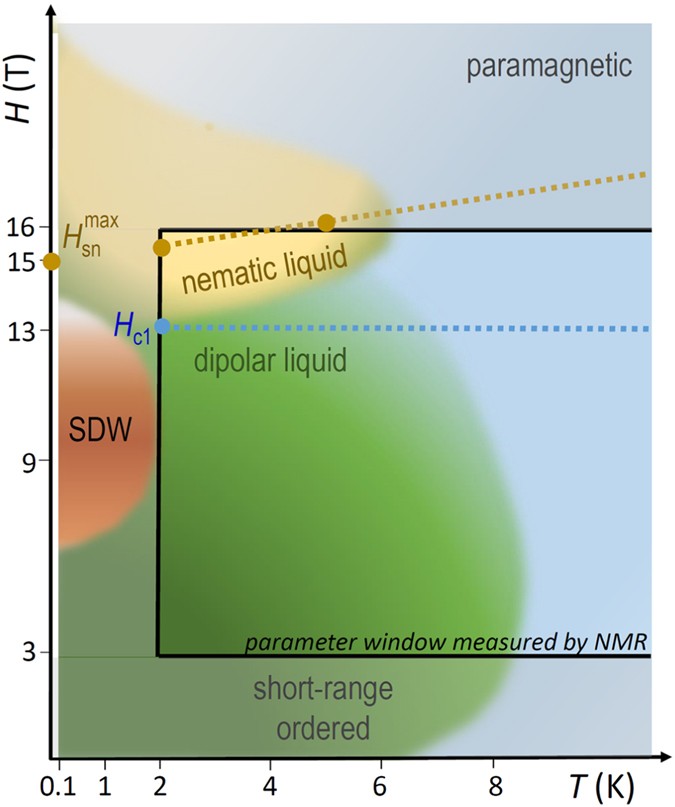
Schematic phase diagram of LiCuSbO4. Blue, dark green, and dark red regions reproduce approximately the diagram of Dutton et al. based on the analysis of the specific heat and magnetization data (Fig. 3 in ref. 26). The dark red area is suggested to present an anomalous SDW phase, whereas the dark yellow area depicts an envisaged stability region of the proposed nematic state. The region measured by the NMR in the present work is marked by the black rectangle. The blue dashed line denotes the isosbestic field H
c1 (cf. Fig. 6). The brown closed circles labelled \({H}_{{\rm{sn}}}^{max}\) connected with the dashed line depict the field of the maximum of the spin-nematic correlation function as found in the DMRG analysis (cf. Fig. 8).
Band structure calculations
As in other related materials (see., e.g., refs 20,21,22 and 27), the edge-sharing geometry of the CuO4 plaquettes in the CuO2 chains in LiCuSbO4 (Fig. 1) is expected to give rise to the usual frustrated magnetism due to the presence of oxygen mediated frustrated AFM NNN intra-chain couplings. The nearly 90° Cu-O-Cu bond angle, i.e. 93°, points to FM NN intra-chain interactions due to the presence of a sizable direct FM coupling K
pd ~ 100 meV between two holes residing on neighboring sites with Cu 3d and O 2p orbitals and a significant compensation of the AFM NN superexchange contributions.
We have performed DFT and DFT+U band structure calculations with the aim to understand (i) the amount of interchain couplings and (ii) the magnitude of the intra-chain couplings. With respect to (i) we have analyzed the dispersion of bands and found pronounced 1D van Hove singularities near the Fermi level. Thus, we have confirmed the nearly 1D behavior of LiCuSbO4. Then, in general, the exchange coupling strength can be estimated simply by the AFM contribution \({J}_{1}=4{t}_{1}^{2}/{U}_{{\rm{eff}}}\), where \({U}_{{\rm{eff}}}\sim {{\rm{\Delta }}}_{pd}\approx 3\) to 4 eV is the effective Coulomb repulsion within a single-band type approach for the Cu-sites with NN transfer integral t
1. The frustrating J
2 is measured by the analogous expression using the NNN transfer integral t
2 instead ignoring a much weaker direct FM contribution as compared to that of the NN bond (\({K}_{pd}\gg {K}_{pp}\)) and the small hole occupation at O 2p orbitals. Note that applying such a simple model to charge transfer insulators as cuprates, one is left with an effective onsite repulsion U of the order of the Cu 3d-O 2p onsite energy difference which is significantly smaller than the U
d ~ 5.5 eV at Cu sites employed in the DFT+U calculations or in more sophisticated five-band pd Hubbard models4 elsewhere. To check this simple first approach, we have determined the Cu-Wannier functions which contain also the essential O 2p contributions. Their tails point to the important coupling directions. In fact, a closer inspection of the crystal structure reveals nonequivalent “left” and “right” NN intra-chain bonds (Fig. 1). This gives rise to alternating NN transfer integrals (\({t}_{1}\ne {t}_{1}^{^{\prime} }\)). The one-band fit results in the following transfer integrals (given in meV): \({t}_{1}=-95.51,\,{t}_{1}^{^{\prime} }=\mathrm{56.44,}\,{t}_{2}=56.96\), and \({t}_{3}=-11.88,\,{t}_{3}^{^{\prime} }=-16.57\). Then the mean NN transfer integral \({\bar{t}}_{1}\) would provide an AFM superexchange contribution to \({J}_{1}^{e}\) for an equidistant chain of about 67 K which for a typical \({J}_{1}^{e}\) of about −80 K like in linarite (see, refs 22 and 47 and references therein) corresponds to an FM contribution of −147 K. As a result we arrive at a sizable splitting of the two NN exchange integrals: \({J}_{1}\approx -160\,{\rm{K}}\) and \({J}_{1}^{^{\prime} }\approx -90\,{\rm{K}}\), whereas J
2 ≈ 37.6 K, only. Thus, within a 1D picture we are left with a dominant FM total NN coupling and an unrenormalized mean frustration parameter \(\bar{\alpha }={J}_{2}/[({J}_{1}+{J}_{1}^{^{\prime} })/2]\sim 0.3\). This value is close to that (α = 0.28) estimated from the fitting of the observed magnetization curve by the DMRG calculations (see below).
Symmetry analysis and the role of DM interactions
The crystal structure of LiCuSbO4 is described by the polar space-group Cmc21
J
1 − J
2 spin-model to describe the chains of the edge-shared CuO4 square-like plaquettes runnning in a-direction. More details of our symmetry analysis are given in the Supplement. In particular, because of the low symmetry, antisymmetric Dzyaloshinskii-Moriya (DM) interactions are allowed for the NN bonds along the spin-chains, \({E}_{D}={{\bf{D}}}_{\nu }\cdot ({{\bf{S}}}_{i}\times {{\bf{S}}}_{i+\nu })\) and have both a homogeneous and a staggered component. These microscopic antisymmetric exchange interactions are caused by the relativistic spin-orbit interactions and compete with the isotropic exchange interactions.
To fit the experimental data for LiCuSbO4, Dutton et al.linear in |D
ν|. However, this could yield an unrealistic picture for the basic magnetic couplings in LiCuSbO4. The determined strength of the effective anisotropic coupling constant is large and would imply an unusual order of magnitude \(|{{\bf{D}}}_{1}|/|{J}_{1}|\sim 1\). The presence of the relativistic antisymmetric exchange in crystals belonging to the crystal classes 2 mm or C
2ν may give rise to two rather different statesinhomogeneous DM couplings’4.
DMRG-calculations
The main aim of this part is to present an analysis of a novel anisotropy mechanism based on the low-symmetric NN exchange anisotropy, which in addition to the J
1 − J
2 frustration, stabilizes a nematic phase in a moderate high-field region to be specified below. We present a first brief analysis also of the effect of weak homogeneous and staggered NN DM couplings which were found not to destroy the nematicity although some weakening has been observed.
Figure 8(a) shows the magnetization curve M(H) measured at T = 0.45 K. Noteworthy, a full saturation is not reached even in the highest accessible field of 20 T. Although this is reminiscent of a typical feature of M(H) at high temperature, the observation temperature is now low enough to prevent a significant finite-temperature effect. To provide a reasonable explanation for this feature, we introduce a 1D frustrated Heisenberg model with an xyz exchange anisotropy and a magnetic field H along the z axis. The Hamiltonian is then given by
$$\begin{array}{rcl} {\mathcal H} & = & \sum _{i,\gamma =x,y,z}\,{J}_{1}^{\gamma }{S}_{i}^{\gamma }{S}_{i+1}^{\gamma }+{J}_{2}\sum _{i}\,{{\bf{S}}}_{i}\cdot {{\bf{S}}}_{i+2}\\ & & +H\sum _{i}\,{S}_{i}^{z},\end{array}$$
(4)
where \({J}_{1}^{\gamma }\) and J
2 are the NN FM and the NNN AFM exchange couplings, respectively, and \({S}_{i}^{\gamma }\) is the γ-component of the spin-operator S
i. When \(H\gg {J}_{1}^{\gamma }\), J
2, by taking the fully polarized FM state as non-perturbative state, its energy is lowered by \({\rm{\Delta }}E={({J}_{1}^{x}-{J}_{1}^{y})}^{2}/\mathrm{[32(}H-{J}_{1}^{z}-{J}_{2})]\) through the second-order process of an individual double spin-flip. Therefore, the magnetization behaves like \({M}_{S}-M\propto {({J}_{1}^{x}-{J}_{1}^{y})}^{2}/H\) at high fields and saturates at its maximum value M
S only at \(H=\infty \), only. We have calculated the magnetization curve using the DMRG technique. By fitting the experimental curve, we have found a possible parameter set: \({J}_{1}^{z}=-546\,{\rm{K}}\), \(({J}_{1}^{x}/{J}_{1}^{z},{J}_{1}^{y}/{J}_{1}^{z})=(1.07,0.99)\), and J
2 = 153 K. Note that these numbers are effective values in the 1D limit, which can be significantly different from the bare values of NN and NNN exchange couplings determined by the DFT+U calculations. Other contributions such as the interchain and longer-range exchange couplings are renormalized into them. As a related similar example we refer the reader to linarite
More interestingly, an exotic nematic state is established by the xyz exchange anisotropy. The xy components of the first term of Eq. (4) can be divided into an exchange term \(\frac{{J}_{1}^{x}+{J}_{1}^{y}}{4}({S}_{i}^{+}{S}_{i+1}^{-}+{h}.{c}\mathrm{.)}\) and a double spin-flip term \(\frac{{J}_{1}^{x}-{J}_{1}^{y}}{4}({S}_{i}^{+}{S}_{i+1}^{+}+h.c\mathrm{.)}\). The latter seems to create an attractive interaction among the parallel spins. Therefore, a 2-magnon bound state, i.e., a nematic state, may be naively expected at high fields in the presence of xyz exchange anisotropy. To check this possibility, we have calculated the nematic correlation function as an indicator of magnon pairing
$$\begin{array}{rcl}{{\mathscr{C}}}_{{\rm{nematic}}} & = & \langle {S}_{i}^{-}{S}_{i+1}^{-}\rangle -\langle {S}_{i}^{-}{S}_{i+\infty }^{-}\rangle \\ & \equiv & \langle {S}_{i}^{+}{S}_{i+1}^{+}\rangle -\langle {S}_{i}^{+}{S}_{i+\infty }^{+}\rangle .\end{array}$$
(5)
Note that this correlation vanishes for lacking xyz exchange anisotropy, because there is no overlap between different S
z sectors. Furthermore, there is an important difference of the two-magnon instability within our unconventional nematicity scenario as compared to the usual isotropic counterpart mentioned above: namely, the total momentum q of a bound two-magnon pair equals to zero just as in a standard BCS superconductor whereas in the isotropic counterpart it equals to q
a = π which resembles the behavior of a Pauli-limited strongly paramagnetic superconductor in an extremely inhomogeneous Fulde-Ferrel-Larkin-Ovchinnikov (FFLO) state. In this context, the recently proposed isotropic multipolar field theory based scenario by Balents and Starykh\(0 < {q}_{a}\ll \pi \) is noteworthy. The present single chain Hamiltonian with the involved specific exchange anisotropy describes a 1D system with a distinctive nematically ordered ground state at T = 0 and at high enough magnetic fields in contrast with simple AFM Heisenberg chains. With increasing finite T this distinct order is more and more suppressed. The stability of the former generalized also to 2D or 3D with respect to interchain couplings and various DM couplings will be investigated in detail in forthcoming work.
The nematic correlation for our parameter set is plotted as a function of H in Fig. 8(b). It is significantly enhanced just above the kink position of the theoretical magnetization curve. This field range with the enhanced correlation agrees well with that region where the spin gap has been experimentally observed, namely, in between μ
0
H = 13–16 T. A similar nematicity scenario has been proposed in our recent work devoted to linarite\({ {\mathcal H} }_{{\rm{DM}}}={\sum }_{i}\,{\bf{D}}\cdot ({{\bf{S}}}_{i}\times {{\bf{S}}}_{i+1})\) with D = (0, 0, γ). As a result we found that the nematic state is hardly affected by a weak DM coupling for γ
0
H = 13 T at T = 0 disappears for higher T which points to existence of the mentioned above upper critical field.
Thus, we are confronted with a somewhat unusual situation: the pronounced spin gap and the strongly enhanced nematic correlations are, in a literal sense, not the result of the occurrence of a novel order parameter associated with symmetry breaking due to a second order phase transition from a high temperature and low-field para-phase, since at low fields the nematic order at T = 0 already exists albeit at a low level. Instead, based on our calculations and in accord with the experimental data, we suggest a crossover from a weak nematic state in a narrow field range at about 13 T to a pronounced nematic state up to at least 16 T to 20 T to be followed by a broad field range where it decreases again (Figs 8 and 9).
Such transitions without a symmetry change of the macroscopic order parameter are reminiscent of mesoscopic liquid-liquid transitions in ordinary liquids such as, for instance, in phosphorus and water. It has been found that those single-component liquids may have different liquid states with distinct correlation functions. A transition between them driven by some external control parameter, such as temperature or pressure, is characterized by the quantitative change of a correlation function, only4, with increasing T these changes are smeared out and the consequences of the suppressed nematic order parameter are difficult to be observed. In such a complex situation further experimental and theoretical studies beyond the scope of the present work are necessary to refine the parameters of our proposed model and to take into account explicitly the weaker couplings and modifications suggested by the real structure including also impurities or defects.


 1万+
1万+


 被折叠的 条评论
为什么被折叠?
被折叠的 条评论
为什么被折叠?
 到【灌水乐园】发言


