python决策树 value_随机森林原理及Python代码

最新推荐文章于 2023-07-23 17:32:00 发布

weixin_39846364

最新推荐文章于 2023-07-23 17:32:00 发布

阅读量425

点赞数

文章标签： python决策树 value 基于python的随机森林回归实现

一、基本原理

随机森林产生的原因：单个决策树对训练数据往往具有较好的分类效果，但是对于未知新样本分类效果较差。为了提升模型对未知样本的分类效果，所以将多个简单的决策树组合起来，形成泛化能力更强的模型——随机森林。

随机森林，名如其实，处处体现着“随机”二字。

随机森林的完整操作过程梳理如下：

（1）首先，从将数据集分为训练集和测试集。

（2）第一个决策树的产生过程如下：

①使用Bootstrap方法从训练集中抽取出一个数据集用于生成第1个决策树。Bootstrap抽样方法随机地从训练集中抽取数据形成新的数据集，并且允许重复抽取同一样本，抽取出的数据集大小等于训练集大小。

②假设有n个变量，每次随机选择2个变量，判断其中的哪个变量更适合做节点，判断依据可以是信息增益、gini指标。通过这种方法先确定决策树的根节点。然后，在剩下的n-1个变量中，继续随机选2个变量，判断谁更适合作为内部节点，并确定内部节点。不断循环，直到生成一棵完整的树。

每次随机选择的变量数可以是3个、4个甚至更多，但如果每次都随机选两个，决策树的生成会更快。

后面的决策树都是循环第①步和第②步产生的。一般来说，随机森林中的决策树棵数为100棵，你也可以生成更多的树。

（3）使用随机森林对新样本（来自测试集）进行分类预测。

假设随机森林中有100棵决策树，那么，我们需要将新样本数据输入到100棵树中，然后，看每棵树返回的分类结果是什么，如果是分类问题，则根据投票原则，少数服从多数来确定新样本最终的类别。如果是回归问题，则取100棵树预测值的均值作为最终的预测值。

如：假设新样本可能有两种类别取值：0和1，使用规模为100的随机森林模型发现，有90棵树预测的类别是1，10棵树预测的结果是0，那么，少数服从多数，新样本的类别会判断为1。

参考：

https://www.youtube.com/watch?v=J4Wdy0Wc_xQwww.youtube.com [中字]简单易懂的随机森林算法原理分析_哔哩哔哩 (゜-゜)つロ干杯~-bilibiliwww.bilibili.com

二、Python实战

练习数据提取地址：https://pan.baidu.com/s/1GAdavxuD9txb57XbuQPzGQ

提取码：yh5a

数据截图：

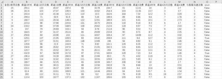
注：isrun为分类标签列，其余列为特征列。

第一步：读入数据

import pandas as pd
path = 'C:UsersCaraDesktopcase.csv'
rawdata = pd.read_csv(path,encoding = 'gbk')#字段名为中文，编码方式指定为gbk
print(rawdata.head())#查看前几行数据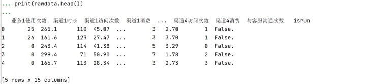

第二步：查看数据基本情况

rawdata.describe()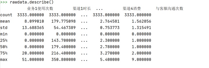

注：isrun列的情况没有反映出来，需要单独查看

#查看目标列（isrun）的频数分布
print(rawdata.isrun.value_counts())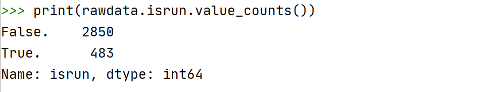

注：①根据dtype可知，False.和True.为int64，即整数型，False.对应0，True.对应1。

②特别注意目标字段（标签列）的数据分布，如果存在某一类记录数特别少，训练出的算法可能预测结果可能会更偏向数量多的那一类，且准确率虚高。

一个极端的例子：总共有100个样本，其中A类样本数量为98条，B类样本数量为2条。现在用50%的样本作为训练集，且按照分层抽样，则抽出的样本集为A类49条，B类样本1条。基于这个训练集进行模型拟合，拟合出的模型自然会倾向于将测试集中的样本预测为A类。事实上，算法将全部测试集均预测为A类也可以，且准确率会相当高。但是，将模型用来预测新的数据集（非测试集）则会大量错判，即模型的泛化能力很差。

面对这种样本类别不均衡的情况，一般来说有两种解决办法：

方法一：在抽样时进行“下抽样”，即以数量较少的那个类别的个数为基准，抽取同等数量的其他类。

第三步：数据处理

#为了便于后续算法运算，将isrun中的FALSE改为0，TRUE改为1
rawdata['isrun'] = rawdata['isrun'].astype(str).map({'False.':0,'True.':1})
print(rawdata.isrun.value_counts())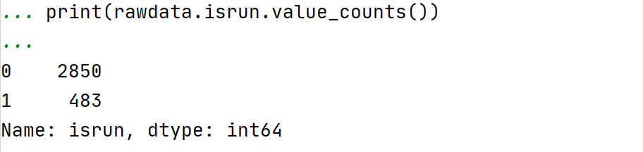

注意：map()函数进行映射时，False及True后面有一个点！

#构造特征集和标签集
x = rawdata.drop('isrun',axis = 1)#删除isrun列，剩余字段全为特征列
y = rawdata['isrun']

#划分出训练集和测试集
from sklearn.model_selection import train_test_split
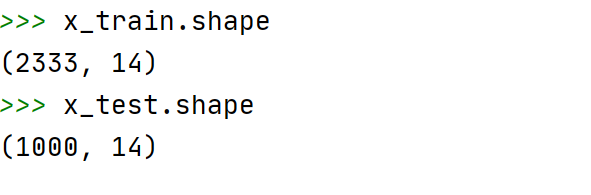
x_train,x_test,y_train,y_test = train_test_split(x,y,test_size = 0.3,random_state=0)#30%为测试集，则70%为训练集
x_train.shape#查看训练集数据量
x_test.shape#查看测试集数据量

第四步：使用随机森林进行分类

Python中随机森林基本参数：

from sklearn.ensemble import RandomForestClassifier
... help(RandomForestClassifier)
... 
Help on class RandomForestClassifier in module sklearn.ensemble._forest:
class RandomForestClassifier(ForestClassifier)
 |  RandomForestClassifier(n_estimators=100, *, criterion='gini', max_depth=None, min_samples_split=2, min_samples_leaf=1, min_weight_fraction_leaf=0.0, max_features='auto', max_leaf_nodes=None, min_impurity_decrease=0.0, min_impurity_split=None, bootstrap=True, oob_score=False, n_jobs=None, random_state=None, verbose=0, warm_start=False, class_weight=None, ccp_alpha=0.0, max_samples=None)
 |  
 |  A random forest classifier.
 |  
 |  A random forest is a meta estimator that fits a number of decision tree
 |  classifiers on various sub-samples of the dataset and uses averaging to
 |  improve the predictive accuracy and control over-fitting.
 |  The sub-sample size is controlled with the `max_samples` parameter if
 |  `bootstrap=True` (default), otherwise the whole dataset is used to build
 |  each tree.
 |  
 |  Parameters
 |  ----------
 |  n_estimators : int, default=100
 |      The number of trees in the forest.
 |  
 |      .. versionchanged:: 0.22
 |         The default value of ``n_estimators`` changed from 10 to 100
 |         in 0.22.
 |  
 |  criterion : {"gini", "entropy"}, default="gini"
 |      The function to measure the quality of a split. Supported criteria are
 |      "gini" for the Gini impurity and "entropy" for the information gain.
 |      Note: this parameter is tree-specific.
 |  
 |  max_depth : int, default=None
 |      The maximum depth of the tree.#树的最大深度
        If None, then nodes are expanded until
 |      all leaves are pure or until all leaves contain less than
 |      min_samples_split samples.
 |  
 |  min_samples_split : int or float, default=2
 |      The minimum number of samples required to split an internal node:
 |  #内部节点如果要被进一步划分，内部节点需要拥有的最小样本数
 |      - If int, then consider `min_samples_split` as the minimum number.
 |      - If float, then `min_samples_split` is a fraction and
 |        `ceil(min_samples_split * n_samples)` are the minimum
 |        number of samples for each split.
 |  
 |      .. versionchanged:: 0.18
 |         Added float values for fractions.
 |  
 |  min_samples_leaf : int or float, default=1
 |      The minimum number of samples required to be at a leaf node.
      #叶子节点最小样本数。
 |      A split point at any depth will only be considered if it leaves at
 |      least ``min_samples_leaf`` training samples in each of the left and
 |      right branches.  This may have the effect of smoothing the model,
 |      especially in regression.
 |  
 |      - If int, then consider `min_samples_leaf` as the minimum number.
 |      - If float, then `min_samples_leaf` is a fraction and
 |        `ceil(min_samples_leaf * n_samples)` are the minimum
 |        number of samples for each node.
 |  
 |      .. versionchanged:: 0.18
 |         Added float values for fractions.
 |  
 |  min_weight_fraction_leaf : float, default=0.0
 |      The minimum weighted fraction of the sum total of weights (of all
 |      the input samples) required to be at a leaf node. Samples have
 |      equal weight when sample_weight is not provided.
 |  
 |  max_features : {"auto", "sqrt", "log2"}, int or float, default="auto"
 |      The number of features to consider when looking for the best split:
 |  
 |      - If int, then consider `max_features` features at each split.
 |      - If float, then `max_features` is a fraction and
 |        `int(max_features * n_features)` features are considered at each
 |        split.
 |      - If "auto", then `max_features=sqrt(n_features)`.
 |      - If "sqrt", then `max_features=sqrt(n_features)` (same as "auto").
 |      - If "log2", then `max_features=log2(n_features)`.
 |      - If None, then `max_features=n_features`.
 |  
 |      Note: the search for a split does not stop until at least one
 |      valid partition of the node samples is found, even if it requires to
 |      effectively inspect more than ``max_features`` features.
 |  
 |  max_leaf_nodes : int, default=None
 |      Grow trees with ``max_leaf_nodes`` in best-first fashion.
 |      Best nodes are defined as relative reduction in impurity.
 |      If None then unlimited number of leaf nodes.
 |  
 |  min_impurity_decrease : float, default=0.0
 |      A node will be split if this split induces a decrease of the impurity
 |      greater than or equal to this value.
 |  
 |      The weighted impurity decrease equation is the following::
 |  
 |          N_t / N * (impurity - N_t_R / N_t * right_impurity
 |                              - N_t_L / N_t * left_impurity)
 |  
 |      where ``N`` is the total number of samples, ``N_t`` is the number of
 |      samples at the current node, ``N_t_L`` is the number of samples in the
 |      left child, and ``N_t_R`` is the number of samples in the right child.
 |  
 |      ``N``, ``N_t``, ``N_t_R`` and ``N_t_L`` all refer to the weighted sum,
 |      if ``sample_weight`` is passed.
 |  
 |      .. versionadded:: 0.19
 |  
 |  min_impurity_split : float, default=None
 |      Threshold for early stopping in tree growth. A node will split
 |      if its impurity is above the threshold, otherwise it is a leaf.
 |  
 |      .. deprecated:: 0.19
 |         ``min_impurity_split`` has been deprecated in favor of
 |         ``min_impurity_decrease`` in 0.19. The default value of
 |         ``min_impurity_split`` has changed from 1e-7 to 0 in 0.23 and it
 |         will be removed in 0.25. Use ``min_impurity_decrease`` instead.
 |  
 |  
 |  bootstrap : bool, default=True
 |      Whether bootstrap samples are used when building trees. If False, the
 |      whole dataset is used to build each tree.
 |  
 |  oob_score : bool, default=False
 |      Whether to use out-of-bag samples to estimate
 |      the generalization accuracy.
 |  
 |  n_jobs : int, default=None
 |      The number of jobs to run in parallel. :meth:`fit`, :meth:`predict`,
 |      :meth:`decision_path` and :meth:`apply` are all parallelized over the
 |      trees. ``None`` means 1 unless in a :obj:`joblib.parallel_backend`
 |      context. ``-1`` means using all processors. See :term:`Glossary
 |      <n_jobs>` for more details.
 |  
 |  random_state : int or RandomState, default=None
 |      Controls both the randomness of the bootstrapping of the samples used
 |      when building trees (if ``bootstrap=True``) and the sampling of the
 |      features to consider when looking for the best split at each node
 |      (if ``max_features < n_features``).
 |      See :term:`Glossary <random_state>` for details.
 |  
 |  verbose : int, default=0
 |      Controls the verbosity when fitting and predicting.
 |  
 |  warm_start : bool, default=False
 |      When set to ``True``, reuse the solution of the previous call to fit
 |      and add more estimators to the ensemble, otherwise, just fit a whole
 |      new forest. See :term:`the Glossary <warm_start>`.
 |  
 |  class_weight : {"balanced", "balanced_subsample"}, dict or list of dicts,             default=None
 |      Weights associated with classes in the form ``{class_label: weight}``.
 |      If not given, all classes are supposed to have weight one. For
 |      multi-output problems, a list of dicts can be provided in the same
 |      order as the columns of y.
 |  
 |      Note that for multioutput (including multilabel) weights should be
 |      defined for each class of every column in its own dict. For example,
 |      for four-class multilabel classification weights should be
 |      [{0: 1, 1: 1}, {0: 1, 1: 5}, {0: 1, 1: 1}, {0: 1, 1: 1}] instead of
 |      [{1:1}, {2:5}, {3:1}, {4:1}].
 |  
 |      The "balanced" mode uses the values of y to automatically adjust
 |      weights inversely proportional to class frequencies in the input data
 |      as ``n_samples / (n_classes * np.bincount(y))``
 |  
 |      The "balanced_subsample" mode is the same as "balanced" except that
 |      weights are computed based on the bootstrap sample for every tree
 |      grown.
 |  
 |      For multi-output, the weights of each column of y will be multiplied.
 |  
 |      Note that these weights will be multiplied with sample_weight (passed
 |      through the fit method) if sample_weight is specified.
 |  
 |  ccp_alpha : non-negative float, default=0.0
 |      Complexity parameter used for Minimal Cost-Complexity Pruning. The
 |      subtree with the largest cost complexity that is smaller than
 |      ``ccp_alpha`` will be chosen. By default, no pruning is performed. See
 |      :ref:`minimal_cost_complexity_pruning` for details.
 |  
 |      .. versionadded:: 0.22
 |  
 |  max_samples : int or float, default=None
 |      If bootstrap is True, the number of samples to draw from X
 |      to train each base estimator.
 |  
 |      - If None (default), then draw `X.shape[0]` samples.
 |      - If int, then draw `max_samples` samples.
 |      - If float, then draw `max_samples * X.shape[0]` samples. Thus,
 |        `max_samples` should be in the interval `(0, 1)`.
 |  
 |      .. versionadded:: 0.22

训练随机森林分类器

from sklearn.ensemble import RandomForestClassifier
rfc = RandomForestClassifier()#使用默认参数将随机森林分类器实例化
rfc.fit(x_train,y_train)#模型拟合

模型评分

#评分方法1：
score1 = rfc.score(x_test,y_test)#查看拟合出的分类器在测试集上的效果
print(score1)
#返回值：0.93
#得分高于0.9，表示预测效果较好。
#评分方法2：
from sklearn.metrics import roc_auc_score
proba = rfc.predict_proba(x_test)#使用分类器预测测试集中每个样本属于0和1的概率
score2 = roc_auc_score(y_test,proba[:,1])
print(score2)
#返回值;0.8439086721140588
#从评价结果来看，默认参数值情况下得到的分类器预测效果还可以

注：①rfc.predict_proba(x_test)表示用分类器预测测试集中每个样本属于0和1的概率。

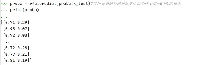
如，[0.71,0.29]表示测试集第一个样本属于类别0的概率为0.71，属于类别1的概率为0.29。根据默认判定规则，在二分类问题中，当样本x属于A类概率大于0.5，则将样本x划分为A类。

②proba[:,1]表示提取每个[]中的第2个元素，即样本属于类别1的概率值。

#评分方法3：
#交叉验证得分
from sklearn.model_selection import cross_val_score
score3 = cross_val_score(rfc,x_train,y_train,scoring='accuracy',cv = 3)#scoring='accuracy'表示评分标准是准确率，cv = 3表示交叉验证的折数为3折。
print(score3)
#返回值：[0.92159383 0.91902314 0.93178893]
#由于cv = 3，因此返回了3个得分

print(score3.mean())#整体平均得分
#返回值：0.9241352994566362

Python中交叉验证得分的帮助文档：

Help on function cross_val_score in module sklearn.model_selection._validation:
cross_val_score(estimator, X, y=None, *, groups=None, scoring=None, cv=None, n_jobs=None, verbose=0, fit_params=None, pre_dispatch='2*n_jobs', error_score=nan)
    Evaluate a score by cross-validation
    
    Parameters
    ----------
    estimator : estimator object implementing 'fit'
        The object to use to fit the data.
    
    X : array-like of shape (n_samples, n_features)
        The data to fit. Can be for example a list, or an array.
    
    y : array-like of shape (n_samples,) or (n_samples, n_outputs),             default=None
        The target variable to try to predict in the case of
        supervised learning.
    
    groups : array-like of shape (n_samples,), default=None
        Group labels for the samples used while splitting the dataset into
        train/test set. Only used in conjunction with a "Group" :term:`cv`
        instance (e.g., :class:`GroupKFold`).
    
    scoring : str or callable, default=None
        A str (see model evaluation documentation) or
        a scorer callable object / function with signature
        ``scorer(estimator, X, y)`` which should return only
        a single value.
    
        Similar to :func:`cross_validate`
        but only a single metric is permitted.
    
        If None, the estimator's default scorer (if available) is used.
    
    cv : int, cross-validation generator or an iterable, default=None
        Determines the cross-validation splitting strategy.
        Possible inputs for cv are:
    
        - None, to use the default 5-fold cross validation,
        - int, to specify the number of folds in a `(Stratified)KFold`,
        - :term:`CV splitter`,
        - An iterable yielding (train, test) splits as arrays of indices.
    
        For int/None inputs, if the estimator is a classifier and ``y`` is
        either binary or multiclass, :class:`StratifiedKFold` is used. In all
        other cases, :class:`KFold` is used.
    
        Refer :ref:`User Guide <cross_validation>` for the various
        cross-validation strategies that can be used here.
    
        .. versionchanged:: 0.22
            ``cv`` default value if None changed from 3-fold to 5-fold.
    
    n_jobs : int, default=None
        The number of CPUs to use to do the computation.
        ``None`` means 1 unless in a :obj:`joblib.parallel_backend` context.
        ``-1`` means using all processors. See :term:`Glossary <n_jobs>`
        for more details.
    
    verbose : int, default=0
        The verbosity level.
    
    fit_params : dict, default=None
        Parameters to pass to the fit method of the estimator.
    
    pre_dispatch : int or str, default='2*n_jobs'
        Controls the number of jobs that get dispatched during parallel
        execution. Reducing this number can be useful to avoid an
        explosion of memory consumption when more jobs get dispatched
        than CPUs can process. This parameter can be:
    
            - None, in which case all the jobs are immediately
              created and spawned. Use this for lightweight and
              fast-running jobs, to avoid delays due to on-demand
              spawning of the jobs
    
            - An int, giving the exact number of total jobs that are
              spawned
    
            - A str, giving an expression as a function of n_jobs,
              as in '2*n_jobs'
    
    error_score : 'raise' or numeric, default=np.nan
        Value to assign to the score if an error occurs in estimator fitting.
        If set to 'raise', the error is raised.
        If a numeric value is given, FitFailedWarning is raised. This parameter
        does not affect the refit step, which will always raise the error.
    
        .. versionadded:: 0.20
    
    Returns
    -------
    scores : array of float, shape=(len(list(cv)),)
        Array of scores of the estimator for each run of the cross validation.

使用默认参数训练出的分类器对测试集进行分类

rfc.predict(x_test)
返回值：
array([0, 0, 0, 0, 1, 0, 0, 0, 0, 0, 0, 0, 0, 0, 1, 0, 0, 0, 0, 0, 0, 0,
       0, 0, 0, 0, 0, 0, 0, 0, 0, 0, 0, 0, 0, 0, 1, 0, 0, 1, 0, 1, 1, 1,
       0, 0, 0, 0, 0, 0, 0, 0, 0, 0, 0, 0, 0, 0, 0, 0, 1, 0, 0, 0, 0, 0,
       0, 0, 0, 0, 0, 0, 1, 0, 0, 1, 0, 0, 0, 0, 0, 0, 0, 0, 0, 0, 0, 0,
       1, 0, 0, 0, 0, 0, 0, 0, 0, 0, 0, 0, 0, 0, 0, 0, 0, 0, 0, 0, 0, 0,
       0, 0, 0, 0, 0, 0, 0, 0, 0, 0, 0, 0, 0, 0, 0, 1, 0, 0, 0, 0, 0, 0,
       0, 0, 0, 0, 0, 0, 1, 0, 0, 0, 1, 0, 0, 0, 0, 0, 0, 0, 0, 0, 0, 0,
       0, 1, 0, 0, 1, 0, 0, 0, 1, 0, 0, 0, 1, 0, 1, 0, 0, 0, 0, 0, 0, 0,
       0, 0, 0, 0, 0, 0, 0, 0, 0, 1, 0, 0, 0, 1, 0, 0, 0, 0, 0, 0, 0, 0,
       0, 0, 0, 0, 0, 0, 0, 0, 0, 0, 0, 1, 0, 0, 1, 0, 0, 0, 0, 0, 0, 0,
       0, 1, 0, 0, 0, 0, 0, 0, 0, 0, 0, 0, 0, 0, 0, 0, 1, 0, 0, 0, 0, 0,
       0, 0, 0, 1, 0, 0, 0, 0, 0, 0, 0, 0, 0, 0, 0, 0, 0, 0, 0, 0, 0, 0,
       0, 0, 0, 0, 0, 0, 0, 0, 0, 0, 1, 0, 0, 0, 0, 0, 0, 0, 0, 0, 0, 0,
       0, 0, 0, 0, 0, 0, 0, 0, 0, 0, 0, 1, 0, 0, 0, 0, 0, 0, 0, 0, 0, 0,
       0, 1, 0, 0, 0, 0, 0, 0, 0, 0, 0, 0, 0, 0, 0, 0, 0, 0, 0, 0, 0, 0,
       0, 0, 1, 0, 1, 0, 0, 0, 0, 1, 0, 0, 0, 1, 0, 0, 0, 0, 0, 0, 0, 0,
       0, 0, 0, 0, 0, 0, 0, 1, 0, 0, 0, 0, 0, 0, 0, 0, 0, 0, 0, 0, 0, 1,
       0, 0, 0, 0, 0, 0, 0, 0, 0, 0, 0, 0, 0, 0, 0, 0, 0, 0, 0, 0, 0, 1,
       1, 0, 0, 0, 0, 0, 0, 0, 0, 0, 0, 0, 0, 0, 1, 0, 0, 0, 0, 0, 0, 0,
       0, 0, 0, 0, 0, 0, 0, 0, 0, 0, 0, 0, 0, 0, 0, 0, 0, 0, 0, 0, 0, 0,
       0, 0, 0, 0, 0, 0, 1, 0, 0, 1, 0, 0, 0, 0, 0, 0, 0, 0, 0, 0, 0, 0,
       0, 0, 0, 0, 0, 1, 0, 0, 0, 0, 0, 0, 0, 0, 0, 0, 0, 0, 0, 0, 0, 0,
       0, 0, 0, 0, 1, 0, 0, 0, 0, 0, 0, 0, 0, 0, 0, 0, 0, 0, 0, 0, 0, 0,
       1, 0, 1, 0, 0, 0, 0, 0, 0, 0, 0, 0, 0, 0, 0, 0, 0, 1, 0, 0, 0, 0,
       0, 0, 0, 0, 0, 0, 0, 0, 0, 0, 0, 0, 0, 0, 1, 0, 0, 0, 0, 0, 0, 0,
       0, 0, 1, 0, 0, 0, 0, 1, 0, 0, 0, 0, 0, 0, 0, 0, 0, 1, 0, 0, 0, 0,
       0, 0, 0, 0, 0, 0, 1, 0, 0, 0, 0, 0, 0, 0, 0, 0, 0, 0, 0, 0, 0, 0,
       0, 0, 0, 0, 0, 0, 0, 0, 0, 0, 0, 0, 0, 0, 1, 0, 0, 1, 0, 0, 1, 0,
       0, 0, 1, 0, 0, 0, 0, 0, 0, 0, 0, 0, 0, 0, 0, 1, 0, 0, 0, 0, 1, 1,
       0, 0, 0, 0, 0, 0, 0, 1, 0, 0, 0, 0, 0, 0, 0, 0, 0, 0, 0, 0, 0, 0,
       0, 0, 0, 0, 0, 0, 0, 0, 0, 0, 0, 0, 0, 1, 0, 0, 0, 0, 0, 0, 0, 1,
       0, 0, 0, 0, 0, 0, 0, 0, 0, 0, 1, 0, 1, 0, 0, 0, 0, 1, 0, 0, 0, 0,
       0, 0, 0, 0, 0, 0, 0, 0, 0, 0, 0, 1, 0, 0, 0, 0, 0, 0, 0, 0, 0, 0,
       0, 0, 0, 0, 0, 1, 0, 0, 1, 0, 0, 0, 0, 0, 0, 0, 0, 0, 0, 0, 0, 0,
       0, 0, 0, 0, 0, 0, 0, 0, 0, 0, 0, 0, 0, 0, 0, 0, 0, 0, 0, 0, 1, 0,
       0, 0, 0, 0, 0, 0, 0, 0, 0, 0, 1, 0, 0, 0, 0, 0, 0, 0, 0, 0, 0, 0,
       0, 0, 0, 0, 0, 0, 0, 0, 0, 0, 0, 0, 0, 0, 0, 0, 0, 0, 1, 0, 0, 0,
       0, 0, 0, 0, 0, 0, 0, 1, 0, 0, 0, 0, 0, 1, 0, 0, 0, 0, 0, 0, 0, 0,
       0, 0, 0, 0, 0, 1, 1, 0, 0, 1, 0, 1, 0, 0, 0, 0, 0, 0, 0, 0, 0, 0,
       0, 0, 0, 0, 0, 0, 0, 0, 0, 0, 1, 0, 0, 0, 0, 0, 0, 0, 0, 0, 0, 0,
       0, 0, 0, 0, 0, 0, 0, 0, 0, 0, 0, 0, 1, 0, 0, 0, 0, 0, 0, 0, 0, 0,
       1, 0, 0, 0, 1, 0, 0, 0, 0, 0, 0, 0, 0, 0, 0, 1, 1, 0, 0, 0, 0, 0,
       0, 0, 0, 0, 0, 0, 0, 0, 0, 0, 0, 0, 0, 0, 0, 0, 0, 0, 0, 0, 0, 0,
       0, 0, 0, 0, 0, 0, 0, 0, 0, 0, 0, 0, 0, 0, 0, 0, 0, 0, 0, 0, 0, 0,
       0, 0, 0, 0, 0, 0, 0, 0, 1, 1, 1, 0, 0, 0, 0, 0, 0, 0, 0, 0, 0, 0,
       0, 0, 0, 0, 0, 0, 0, 0, 0, 0], dtype=int64)

查看该分类器计算出的每个特征列在分类上的重要性：

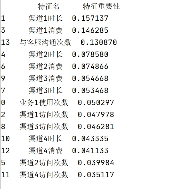
importance

注：np.array(col)[:-1]表示将col转换为array格式，并且扔掉最后一个元素（isrun）。

结果如下：

第五步：参数调优

参数调优的基本策略是，一次调一个参数，将该参数固定下来，再调下一个参数。

#（1）将随机森林分类器rfc中第一个参数n_estimators调至最优。
from sklearn.model_selection import GridSearchCV
num_estimator = {'n_estimators':range(50,300,50)}#随机森林中树的棵数，以50为起点，50为步长，最多为300棵树
gs1 = GridSearchCV(estimator = rfc,param_grid = num_estimator,scoring='roc_auc',cv = 3)
gs1.fit(x_train,y_train)
print(gs1.best_estimator_)#查看最佳分类器
#返回值：RandomForestClassifier(n_estimators=200)
print(gs1.best_score_)#查看最佳分类器对应的得分
#返回值：0.8634028368426186
#这里的得分是一个均值，由于设置了cv = 3，因此是3次交叉验证得分的均值

#（2）将n_estimators固定为最优值（200），然后再调树的最大深度max_depth
maxdepth = {'max_depth':range(3,10,1)}
gs2 = GridSearchCV(estimator = RandomForestClassifier(n_estimators = 200),param_grid = maxdepth,scoring = 'roc_auc',cv = 3)
gs2.fit(x_train,y_train)
print(gs2.best_estimator_)#查看最佳分类器
#返回值：RandomForestClassifier(max_depth=8, n_estimators=200)
print(gs2.best_score_)#查看最佳分类器对应的得分
#返回值：0.864779319225661
#可见，最佳分类器得分略有提升

#（3）max_depth=8, n_estimators=200固定不变，继续调min_samples_split
minsamples = {'min_samples_split':range(2,50,2)}
gs3 = GridSearchCV(estimator = RandomForestClassifier(max_depth=8, n_estimators=200),param_grid = minsamples,scoring = 'roc_auc',cv = 3)
gs3.fit(x_train,y_train)
print(gs3.best_estimator_)#查看最佳分类器
#返回值：RandomForestClassifier(max_depth=8, min_samples_split=16, n_estimators=200)
print(gs3.best_score_)#查看最佳分类器对应的得分
#返回值：0.8635835529670378
#额，得分不升反降啊！参数调优是个艺术活……

基于最优的参数进行预测

best_rfc = RandomForestClassifier(max_depth=8, min_samples_split=16, n_estimators=200)
best_rfc.fit(x_train,y_train)
print(best_rfc.score(x_test,y_test))
#返回值：0.924
best_rfc.predict(x_test)
#返回值：
array([0, 0, 0, 0, 1, 0, 0, 0, 0, 0, 0, 0, 0, 0, 1, 0, 0, 0, 0, 0, 0, 0,
       0, 0, 0, 0, 0, 0, 0, 0, 0, 0, 0, 0, 0, 0, 1, 0, 0, 1, 0, 1, 1, 1,
       0, 0, 0, 0, 0, 0, 0, 0, 0, 0, 0, 0, 0, 0, 0, 0, 1, 0, 0, 0, 0, 0,
       0, 0, 0, 0, 0, 0, 1, 0, 0, 1, 0, 0, 0, 0, 0, 0, 0, 0, 0, 0, 0, 0,
       1, 0, 0, 0, 0, 0, 0, 0, 0, 0, 0, 0, 0, 0, 0, 0, 0, 0, 0, 0, 0, 0,
       0, 0, 0, 0, 0, 0, 0, 0, 0, 0, 0, 0, 0, 0, 0, 1, 0, 0, 0, 0, 0, 0,
       0, 0, 0, 0, 0, 0, 1, 0, 0, 0, 1, 0, 0, 0, 0, 0, 0, 0, 0, 0, 0, 0,
       0, 1, 0, 0, 1, 0, 0, 0, 1, 0, 0, 0, 1, 0, 1, 0, 0, 0, 0, 0, 0, 0,
       0, 0, 0, 0, 0, 0, 0, 0, 0, 1, 0, 0, 0, 1, 0, 0, 0, 0, 0, 0, 0, 0,
       0, 0, 0, 0, 0, 0, 0, 0, 0, 0, 0, 1, 0, 0, 1, 0, 0, 0, 0, 0, 0, 0,
       0, 1, 0, 0, 0, 0, 0, 0, 0, 0, 0, 0, 0, 0, 0, 0, 1, 0, 0, 0, 0, 0,
       0, 0, 0, 1, 0, 0, 0, 0, 0, 0, 0, 0, 0, 0, 0, 0, 0, 0, 0, 0, 0, 0,
       0, 0, 0, 0, 0, 0, 0, 0, 0, 0, 1, 0, 0, 0, 0, 0, 0, 0, 0, 0, 0, 0,
       0, 0, 0, 0, 0, 0, 0, 0, 0, 0, 0, 1, 0, 0, 0, 0, 0, 0, 0, 0, 0, 0,
       0, 1, 0, 0, 0, 0, 0, 0, 0, 0, 0, 0, 0, 0, 0, 0, 0, 0, 0, 0, 0, 0,
       0, 0, 1, 0, 0, 0, 0, 0, 0, 1, 0, 0, 0, 1, 0, 0, 0, 0, 0, 0, 0, 0,
       0, 0, 0, 0, 0, 0, 0, 1, 0, 0, 0, 0, 0, 0, 0, 0, 0, 0, 0, 0, 0, 1,
       0, 0, 0, 0, 0, 0, 0, 0, 0, 0, 0, 0, 0, 0, 0, 0, 0, 0, 0, 0, 1, 1,
       1, 0, 0, 0, 0, 0, 0, 0, 0, 0, 0, 0, 0, 0, 1, 0, 0, 0, 0, 0, 0, 0,
       0, 0, 0, 0, 0, 0, 0, 0, 0, 0, 0, 0, 0, 0, 0, 0, 0, 0, 0, 0, 0, 0,
       0, 0, 0, 0, 0, 0, 1, 0, 0, 1, 0, 0, 0, 0, 0, 0, 0, 0, 0, 0, 0, 0,
       0, 0, 0, 0, 0, 1, 0, 0, 0, 0, 0, 0, 0, 0, 0, 0, 0, 0, 0, 0, 0, 0,
       0, 0, 0, 0, 0, 0, 0, 0, 0, 0, 0, 0, 0, 0, 0, 0, 0, 0, 0, 0, 0, 0,
       1, 0, 1, 0, 0, 0, 0, 0, 0, 0, 0, 0, 0, 0, 0, 0, 0, 1, 0, 0, 0, 0,
       0, 0, 0, 0, 0, 0, 0, 0, 0, 0, 0, 0, 0, 0, 1, 0, 0, 0, 0, 0, 0, 0,
       0, 0, 1, 0, 0, 0, 0, 0, 0, 0, 0, 0, 0, 0, 0, 0, 0, 1, 0, 0, 0, 0,
       0, 0, 0, 0, 0, 0, 1, 0, 0, 0, 0, 0, 0, 0, 0, 0, 0, 0, 0, 0, 0, 0,
       0, 0, 0, 0, 0, 0, 0, 0, 0, 0, 0, 0, 0, 0, 0, 0, 0, 1, 0, 0, 1, 0,
       0, 0, 1, 0, 0, 0, 0, 0, 0, 0, 0, 0, 0, 0, 0, 1, 0, 0, 0, 0, 1, 1,
       0, 0, 0, 0, 0, 0, 0, 1, 0, 0, 0, 0, 0, 0, 0, 0, 0, 0, 0, 0, 0, 0,
       0, 0, 0, 0, 0, 0, 0, 0, 0, 0, 0, 0, 0, 1, 0, 0, 0, 1, 0, 0, 0, 1,
       0, 0, 0, 0, 0, 0, 0, 0, 0, 0, 1, 0, 1, 0, 0, 0, 0, 1, 0, 0, 0, 0,
       0, 0, 0, 0, 0, 0, 0, 0, 0, 0, 0, 1, 0, 0, 0, 0, 0, 0, 0, 0, 0, 0,
       0, 0, 0, 0, 0, 1, 0, 0, 1, 0, 0, 0, 0, 0, 0, 0, 0, 0, 0, 0, 0, 0,
       0, 0, 0, 0, 0, 0, 0, 0, 0, 0, 0, 0, 0, 0, 0, 0, 0, 0, 0, 0, 1, 0,
       0, 0, 0, 0, 0, 0, 0, 0, 0, 0, 1, 0, 0, 0, 0, 0, 0, 0, 0, 0, 0, 0,
       0, 0, 0, 0, 0, 0, 0, 0, 0, 0, 0, 0, 0, 0, 0, 0, 0, 0, 1, 0, 0, 0,
       0, 0, 0, 0, 0, 0, 0, 1, 0, 0, 0, 0, 0, 1, 0, 0, 0, 0, 0, 0, 0, 0,
       0, 0, 0, 0, 0, 0, 1, 0, 0, 1, 0, 1, 0, 0, 0, 0, 0, 0, 0, 0, 0, 0,
       0, 0, 0, 0, 0, 0, 0, 0, 0, 0, 1, 0, 0, 0, 0, 0, 0, 0, 0, 0, 0, 0,
       0, 0, 0, 0, 0, 0, 0, 0, 0, 0, 0, 0, 1, 0, 0, 0, 0, 0, 0, 0, 0, 0,
       1, 0, 0, 0, 1, 0, 0, 0, 0, 0, 0, 0, 0, 0, 0, 1, 1, 0, 0, 0, 0, 0,
       0, 0, 0, 0, 0, 0, 0, 0, 0, 0, 0, 0, 0, 0, 0, 0, 0, 0, 0, 0, 0, 0,
       0, 0, 0, 0, 0, 0, 0, 0, 0, 0, 0, 0, 0, 1, 0, 0, 0, 0, 0, 0, 0, 0,
       0, 0, 0, 0, 0, 0, 0, 0, 1, 1, 1, 0, 0, 0, 0, 0, 0, 0, 0, 0, 0, 0,
       0, 0, 0, 0, 0, 0, 0, 0, 0, 0], dtype=int64)

附全部代码：

import pandas as pd
path = 'C:UsersCaraDesktopcase.csv'
rawdata = pd.read_csv(path,encoding = 'gbk')#字段名为中文，编码方式指定为gbk
print(rawdata.head())#查看前几行数据

#查看数据基本情况
rawdata.describe()

#查看目标列（isrun）的频数分布
print(rawdata.isrun.value_counts())

#为了便于后续算法运算，将isrun中的FALSE改为0，TRUE改为1
rawdata['isrun'] = rawdata['isrun'].astype(str).map({'False.':0,'True.':1})
print(rawdata.isrun.value_counts())

#构造特征集和标签集
x = rawdata.drop('isrun',axis = 1)
y = rawdata['isrun']

#划分出训练集和测试集
from sklearn.model_selection import train_test_split
x_train,x_test,y_train,y_test = train_test_split(x,y,test_size = 0.3,random_state=0)
x_train.shape#查看训练集数据量
x_test.shape#查看测试集数据量

#使用随机森林进行分类
from sklearn.ensemble import RandomForestClassifier
rfc = RandomForestClassifier()#使用默认参数将随机森林分类器实例化
rfc.fit(x_train,y_train)#模型拟合

#模型效果评价
#评分方法1：
score1 = rfc.score(x_test,y_test)#查看拟合出的分类器在测试集上的效果
print(score1)

#评分方法2：
from sklearn.metrics import roc_auc_score
proba = rfc.predict_proba(x_test)#使用分类器预测测试集中每个样本属于0和1的概率
score2 = roc_auc_score(y_test,proba[:,1])
print(score2)

#评分方法3：
from sklearn.model_selection import cross_val_score
score3 = cross_val_score(rfc,x_train,y_train,scoring='accuracy',cv = 3)
print(score3)
print(score3.mean())#整体平均得分

#预测
rfc.predict(x_test)#使用分类器预测测试集的类别

#特征重要性
importance = rfc.feature_importances_#查看各个特征列的重要性
col = rawdata.columns#查看数据框的全部字段名（包括isrun）,返回格式为Index
import numpy as np
re = pd.DataFrame({'特征名':np.array(col)[:-1],'特征重要性':importance}).sort_values(by = '特征重要性',axis = 0,ascending = False)
print(re)

#参数调优
#先调n_estimators，即随机森林中树的棵数
from sklearn.model_selection import GridSearchCV
num_estimator = {'n_estimators':range(50,300,50)}#随机森林中树的棵数，以50为起点，50为步长，最多为300棵树
gs1 = GridSearchCV(estimator = rfc,param_grid = num_estimator,scoring = 'roc_auc',cv = 3)
gs1.fit(x_train,y_train)
print(gs1.best_estimator_)#查看最佳分类器对应的得分
print(gs1.best_score_)#查看最佳分类器对应的得分

#将n_estimators固定为最优值（200），然后再调树的最大深度max_depth
maxdepth = {'max_depth':range(3,10,1)}
gs2 = GridSearchCV(estimator = RandomForestClassifier(n_estimators = 200),param_grid = maxdepth,scoring = 'roc_auc',cv = 3)
gs2.fit(x_train,y_train)
print(gs2.best_estimator_)#查看最佳分类器
print(gs2.best_score_)#查看最佳分类器对应的得分

#max_depth=8, n_estimators=200固定不变，继续调min_samples_split
minsamples = {'min_samples_split':range(2,50,2)}
gs3 = GridSearchCV(estimator = RandomForestClassifier(max_depth=8, n_estimators=200),param_grid = minsamples,scoring = 'roc_auc',cv = 3)
gs3.fit(x_train,y_train)
print(gs3.best_estimator_)#查看最佳分类器
print(gs3.best_score_)#查看最佳分类器对应的得分

#基于最优的参数进行预测
best_rfc = RandomForestClassifier(max_depth=8, min_samples_split=16, n_estimators=200)#使用最优参数对随机森林进行类的实例化
best_rfc.fit(x_train,y_train)#模型拟合
print(best_rfc.score(x_test,y_test))#查看best_rfc在测试集上的得分
best_rfc.predict(x_test)#对测试集样本进行分类

参考：

随机森林Python实战_哔哩哔哩 (゜-゜)つロ干杯~-bilibiliwww.bilibili.com

weixin_39846364

关注

0
点赞
踩
1

收藏

觉得还不错? 一键收藏
0
评论
python决策树 value_随机森林原理及Python代码

一、基本原理随机森林产生的原因：单个决策树对训练数据往往具有较好的分类效果，但是对于未知新样本分类效果较差。为了提升模型对未知样本的分类效果，所以将多个简单的决策树组合起来，形成泛化能力更强的模型——随机森林。随机森林，名如其实，处处体现着“随机”二字。随机森林的完整操作过程梳理如下：（1）首先，从将数据集分为训练集和测试集。（2）第一个决策树的产生过程如下：①使用Bootstrap方法从训练集中...
复制链接

扫一扫