python train 函数_机器学习：Logistic回归解释及Python实现

在本文中，我们将深入研究机器学习中的广义线性回归模型来进行分类而不是预测。机器学习中的逻辑回归被称为线性分类器。它计算两个类在0和1之间的概率。如果一个项目的概率分数小于0.5，我们可以简单地对它进行分类，分类到Class 1，否则分类到Class 2。

为了得到逻辑回归的公式，由于它在概率模型上工作，我们必须通过logit(log odds)给出线性方程的值。

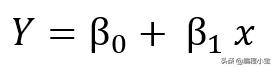
线性模型由下式给出：

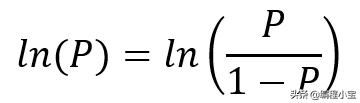
Logit：

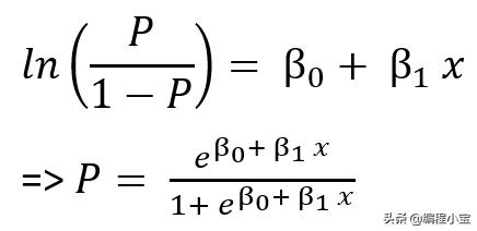
Logistic回归公式由下式给出：

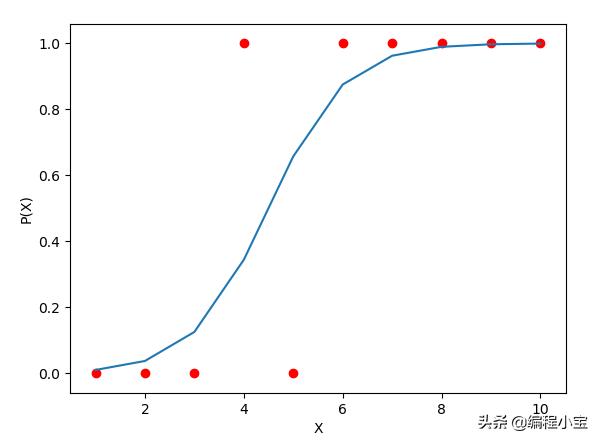
由logistic回归形成的图形如下图所示，通常为“s”形，y轴上的值始终在0 - 1之间:

现在我们必须找到β0和β1的值，但是像线性回归一样，没有这样直接的公式来计算系数。这些系数的估计方法有很多种，如极大似然法、对数似然法、Newton Raphson法等。

Newton Raphson法

Newton Raphson方法是泰勒展开的迭代过程，用于找到图的根，根是图与x轴相交的点，这是我们的系数之一。系数可以通过Newton Raphson方法给出：

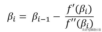
βi是系数的估计值之一，βi-1是在最后一次迭代中估计的相同系数的值。我们将迭代相同的过程直到βi的值稳定。现在我们需要找到函数的一阶和二阶导数。

伯努利分布的似然函数：

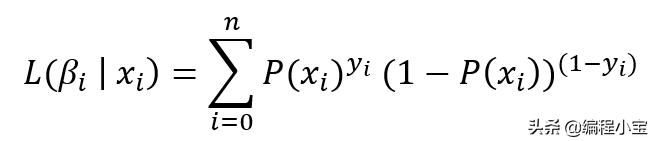
注意：我可以用上面等式中的P值替换它并将其设置为零，如果我这样做，我可以通过找出β0和β1函数的最大值来估计β0和β1的值。这种方法称为最大似然法。但是找到这样的值将非常困难，或者我们可能无法估计正确的值。现在用log来化简这个方程：

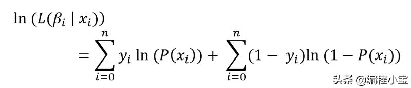
代入P值并化简

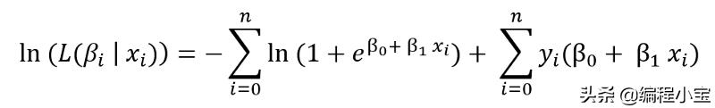
现在，一阶导数是

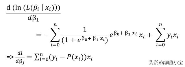
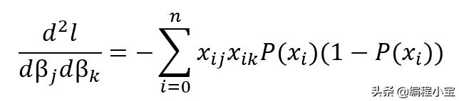
注意：我们可以将上面的等式设置为零，并尝试找出β0和β1的值，该方法称为对数似然法。但同样，我们将无法将其设置为零并解决它，因此采用二阶导数并进行generalizing：

Python实现

我们已经推导出了概率函数，一阶导数和二阶导数。让我们进入python来实现同样的功能。创建一个logsticregression类，并添加如下方法，Python实现如下:

class LogisticRegression: def __init__(self, X): self.beta_old_i = [] #initializing b_i, always one additional coefficient than number of features of predictor #because eq β_0 + β_1*x having two coefficients β_0, β_1 where x has only one dimension self.beta_new_i = np.zeros(X.shape[1] + 1)  #p(x) = e^(β_0 + β_1*x)/(1 + e^(β_0 + β_1*x)) def probabilityFun(self, X): z = np.dot(self.beta_new_i, X.T) p = math.e**z/(1 + math.e**z) return p#f'(β_j) = dl/d(β_j) = (i=1 to N)_Σ (y_i - p(x_i))*x_ij def firstDerivative(self, X, Y, P): firstDer = np.dot((Y-P), X) return firstDer#f''(β_k) = dl/d(β_j)d(β_k) = - (i=1 to N)_Σ x_ij*x_ik*p(x_i)*(1 - p(x_i)) def secondDerivative(self, X, P): probMul = P*(1-P) xMulp = np.array([x*y for (x,y) in zip(X, probMul)]) secondDer = -1*np.dot(xMulp.T,X) return secondDer#β_(i+1) = β_i - (f'(β_i))/(f''(β_i)) def newtonRaphson(self, firstDer, secondDer): self.beta_new_i = self.beta_old_i - np.dot(linalg.inv(secondDer), firstDer)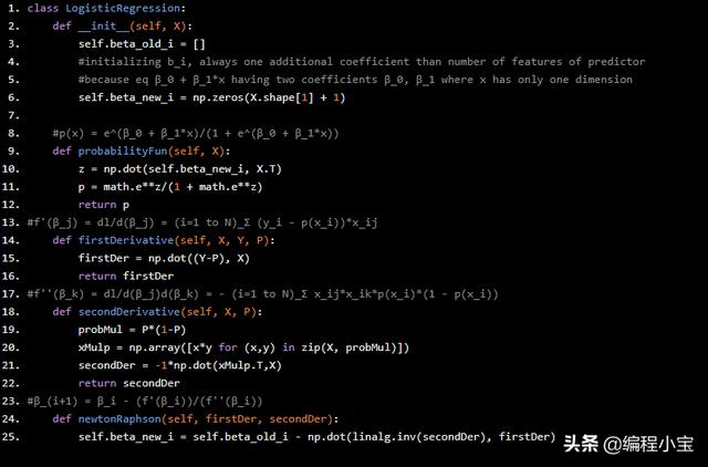

所有函数都是按照导出的公式定义的。现在我们来写一个迭代过程，直到系数稳定下来。Python代码如下：

#training the modeldef fit(self, X, Y, maxIteration=50, diffThreshHold=10**-5): #adding one additional column since we will have additional coefficient X = np.c_[X, np.array([1]*X.shape[0])] iteration = 0 diffBetaList = []while(list(self.beta_new_i) != list(self.beta_old_i)): self.beta_old_i = self.beta_new_i P = self.probabilityFun(X) firstDer = self.firstDerivative(X, Y, P) secondDer = self.secondDerivative(X, P) self.newtonRaphson(firstDer, secondDer) #difference between last calcuated coefficients and current coefficients diff = linalg.norm(self.beta_new_i - self.beta_old_i) diffBetaList.append(diff) iteration += 1 if(diff <= diffThreshHold or iteration > maxIteration): break  return diffBetaList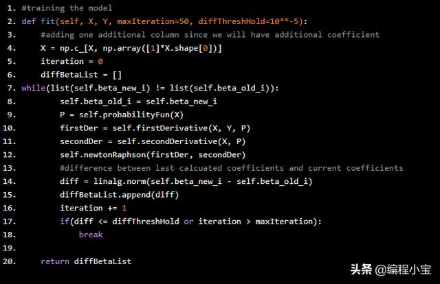

现在创建一个预测和分类方法来计算概率和分类。Python代码如下：

#predict probability any new data pointsdef predict(self, X): X = np.c_[X, np.array([1]*X.shape[0])] probability = self.probabilityFun(X) return probability#classify based on provided classesdef classify(self, X, dataClass): Y = self.predict(X) #if probability is less than 0.5 than categorized as class one else class two return [0 if item <= 0.05 else 1 for item in Y]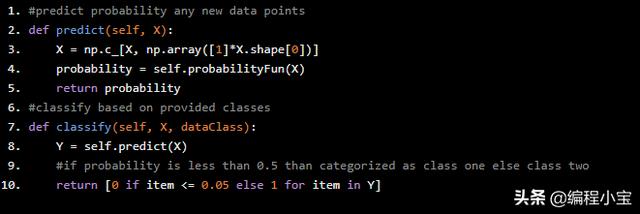

最后使用iris数据训练和测试上面的代码，我将只使用两类iris数据：

iris = datasets.load_iris()#iris data is 50 each three classes so only taking to 100 for two classesx_train, x_test, y_train, y_test = train_test_split(iris['data'][:100], iris['target'][:100])reg = LogisticRegression(x_train)reg.fit(x_train,y_train)pred = reg.classify(x_test, iris["target_names"][:2])print("Accuracy: {:.2f}%".format(100*np.mean(pred == y_test)))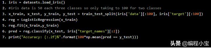

Output

Accuracy: 100.00%