mfc倾斜文本输入_一文弄懂文本检测算法Corner（附源码）

论文在Multi-Oriented Scene Text Detection via Corner Localization and Region Segmentation，CVPR 2018入选文章，看白翔老师很推荐（虽然论文作者都与白翔老师有千丝万缕的联系），效果也很棒：

相应的开源代码在lvpengyuan/corner。

欣慰的一点是文本识别依旧用CRNN，感觉路子没有走偏。

论文作者的介绍文章：旷视科技：CVPR 2018 | 旷视科技Face++新方法——通过角点定位和区域分割检测场景文本

---

0 Abstract

之前的文本检测分为两类：一类是源于通用物体检测的边界回归算法，缺点是文本不是典型的通用物体（方向随机以及长宽比过大或过小），一类是源于语义分割，缺点是需要复杂的后处理算法：

The first category treats scene text as a type of general objects and follows general object detection paradigm to localize scene text by regressing the text box locations, but troubled by the arbitrary-orientation and large aspect ratios of scene text. The second one segments text regions directly, but mostly needs complex post processing.

Corner结合了这两类算法的优点，相应的避免了他们的缺点。

ps:我认为论文讲的还是有些含蓄，文本不是典型的通用物体原因之一在于文本的长宽比过大或过小，那么过大或过小的原因是什么？具体到通用物体检测，你见过这么长的猫吗：

一般的物体（比如猫、狗）由头、身子、尾巴等几个属性不同的元素组成，而不同元素之间又有比例上的关系导致其长宽比不会过大，这导致其子集合很少可以称之为该物体（只有一个头的猫你怕不怕）。

但文本不同，其组成元素属性是相同的，都是单个的字符。因此，文本的子集合也可以称之为文本，甚至单个字符也可以称之为文本。

这其实带给我一些思考，就是文本框的检测第一步最好不要一步到位，我们只需要预测文本的局部，通过组合仍然可以组成长文本，但是一步到位的检测网络可能会导致其在长文本检测上困难相对更大。

这也是我认为论文检测角点的出发点所在，另外一个我觉得有此思想的就是CTPN了。

---

1. Introduction

文本检测会有诸如任意朝向，长宽比不定，文本可以是字符，词，句子等困难：

Compared with general object detection, scene text detection is more complicated because: 1) Scene text may exist in natural images with arbitrary orientation, so the bounding boxes can also be rotated rectangles or quadrangles; 2) The aspect ratios of bounding boxes of scene text vary significantly; 3) Since scene text can be in the form of characters, words, or text lines, algorithms might be confused when locating the boundaries.

针对第一个困难，文本是任意朝向的，这里假设朝向角度位于[-45度,45度]的区间内（现实中大部分的文本也分布在这个区间），我能想到的一个问题就是文本检测和文本识别的分工问题，文本识别也是可以识别倾斜文字的啊，这是我的一个疑问。

论文敢于结合两类算法的底气来于两个发现：一是矩形可以顶点表示，这种表示可以不管矩形尺寸、长宽比和方向；二是语义分割图可以提供文本的有效信息。

算法概览图：

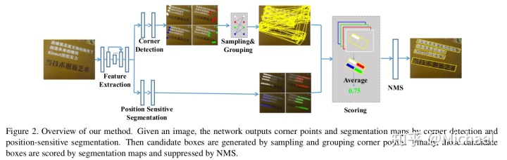
大致思路是用角点的组合生成候选框，使用语义分割图的信息来辅助判断候选框的好坏。

---

2. Related Work

没啥好讲的。

---

3. Network

网络如下：

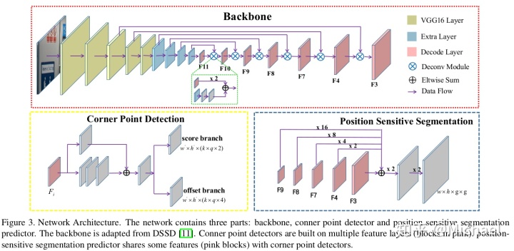
分为3个部分：作为主干网络的特征提取网络、Corner Detection、Position-Sensitive Segmentation。

3.1. Feature Extraction

主支有两个操作，先是卷积操作，然后是反卷积操作，结果就是特征层尺寸先减小后增大。

为了更好实现小目标的检测，除了需要利用反卷积增大特征层尺寸，还需要将低阶的特征图加到高阶的反卷积特征图上：

Particularly, to detect text with different sizes well, we cascade deconvolution modules with 256 channels from conv11 to conv3 (the features from conv10, conv9, conv8, conv7, conv4, conv3 are reused), and 6 deconvolution modules are built in total.

有些参数论文之后会叙述，首先是输入尺寸，训练的输入尺寸在5.2节中明示了，强制resize到512*512：

We randomly sample a patch from the input image in the manner of SSD, then resize the sampled patch to 512*512.

代码里通过构造数据集来resize输入图片，在corner/train.py里这样构造MLT数据集：

dataset = MLTDetection(args.mlt_root, 'train', SSDAugmentation(
        (512, 512), means), AnnotationTransform())
data_loader = data.DataLoader(dataset, batch_size, num_workers=args.num_workers,
                                 shuffle=True, collate_fn=detection_collate, pin_memory=True)

类MLTDetection()使用了默认尺寸dim=(512, 512)，但这个resize只是对非train情况（test等）：

if self.split != 'train':
     img = cv2.resize(img, (self.dim[1], self.dim[0])).astype(np.float64)
     img -= np.array([104.00698793, 116.66876762, 122.67891434])  ## mean -bgr
     img = img[:, :, (2, 1, 0)] ## rgb
     return torch.from_numpy(img).permute(2, 0, 1).float(), img_path, height, width

由于要实现数据增强，使用类SSDAugmentation()来完成数据增强和resize的工作：

class SSDAugmentation(object):
    def __init__(self, size=(512, 512), mean=(104, 117, 123)):
        self.mean = mean
        self.size = size
        self.augment = Compose([
            ConvertFromInts(),
            # ToAbsoluteCoords(),
            PhotometricDistort(),
            Expand(self.mean),
            RandomSampleCrop(),
            RandomMirror(),
            
            ToPercentCoords(),
            Resize(self.size),

            # ToAbsoluteCoords(),
            # RandomRotate(),
            # ToPercentCoords(),
            
            SubtractMeans(self.mean)
        ])

可以看到其中实现了mirror、resize、substract means等操作。

对Test的情况，论文在5.3节中指出，会设置多种比例的图片来评估模型，这种情况在评价结果表（比如表2）使用*表示多尺寸：

In testing, we set

to 0.7 and resize the input images to

. Following [53, 17, 16], we also evaluate our model on ICDAR2015 with multi-scale inputs, {

,

,

,

} in default.

对应的代码在corner/eval_all.py，通过设置传入参数version来设置test图片的大小。

检测的时候也可以使用

这个单尺寸。

为了分析方便，这里只以训练尺寸即512*512来分析网络。

网络的生成代码是这样的：

dssd_net = build_dssd('train', train_cfg, ssd_dim,2)

这个类是这样的：

def build_dssd(phase, cfg, size=512, num_classes=2):
    base_net, extras_submodels, head = multibox(vgg(base[str(size)], 3), add_extras(extras[str(size)], 1024), mbox['512'], 2)
    return DSSD(phase, base_net, extras_submodels, head, deconv_modules(dm), predict_modules(pm), seg_modules(sm), cfg)

主干网络的定义在：

vgg(base[str(size)], 3)

vgg是这么定义的：

# This function is derived from torchvision VGG make_layers()
# https://github.com/pytorch/vision/blob/master/torchvision/models/vgg.py
def vgg(cfg, i, batch_norm=False):
    layers = []
    in_channels = i
    for v in cfg:
        if v == 'M':
            layers += [nn.MaxPool2d(kernel_size=2, stride=2)]
        elif v == 'C':
            layers += [nn.MaxPool2d(kernel_size=2, stride=2, ceil_mode=True)]
        else:
            conv2d = nn.Conv2d(in_channels, v, kernel_size=3, padding=1)
            if batch_norm:
                layers += [conv2d, nn.BatchNorm2d(v), nn.ReLU(inplace=True)]
            else:
                layers += [conv2d, nn.ReLU(inplace=True)]
            in_channels = v
    pool5 = nn.MaxPool2d(kernel_size=3, stride=1, padding=1)
    conv6 = nn.Conv2d(512, 1024, kernel_size=3, padding=6, dilation=6)
    conv7 = nn.Conv2d(1024, 1024, kernel_size=1)
    layers += [pool5, conv6,
               nn.ReLU(inplace=True), conv7, nn.ReLU(inplace=True)]
    return layers

那么，可以看出base[str(size)]定义的是VGG16网络，也就是for v in cfg这段循环，"M"和"C"的区别在于ceil_mode是否为True（ceil_mode可参考Pytorch(2) maxpool的ceil_mode，类似于TensorFlow中padding的作用），对输入为512是没有作用的，这里猜测是为test的多种输入相关。

这里size为512，base是一个字典：

base = {
    '512': [64, 64, 'M', 128, 128, 'M', 256, 256, 256, 'C', 512, 512, 512, 'M',
            512, 512, 512],
}

可以看到有4个maxpool，512的输出经过4个maxpool的尺寸依次变为256、128、64、32。

之后经过pool5，参考torch.nn - PyTorch master documentation及Pytorch(1) pytorch和tensorflow里面的maxpool，Pytorch里面padding是两端补齐的，因此得到的尺寸为：

这里padding的作用是补齐，因此pool5输出的尺寸为32。

之后会有两个卷积操作conv6、conv7，参考torch.nn - PyTorch master documentation及pytorch的函数中的dilation参数的作用 - 慢行厚积 - 博客园，设置dilation为6的目的在于引入空洞卷积，符合论文扩大感受野的目的，这里计算尺寸为：

conv7是经典的1*1卷积，目的在于重组信息。

有了列表，加入到网络是在类DSSD()中的forward()函数里的：

# apply vgg up to conv3_3 relu 256
for k in range(16):
    x = self.vgg[k](x)
sources.append(x)

for k in range(16, 23):
    x = self.vgg[k](x)
# s = self.L2Norm(x)
# sources.append(s)
sources.append(x)

# apply vgg up to fc7
for k in range(23, len(self.vgg)):
    x = self.vgg[k](x)
sources.append(x)

注意这里使用了3个锚点（即conv3、conv4、conv7，注意每个卷积在vgg列表里占了2个，即卷积加ReLU），放到列表sources里面去，这是为了之后反卷积操作使用的。

另外，还有Extra Layer用于扩大感受野：

Then several extra convolutional layers (conv8, conv9, conv10, conv11) are stacked above conv7 to enlarge the receptive fields of extracted features.

对应的代码是：

add_extras(extras[str(size)], 1024)

而add_extras()函数为：

def add_extras(cfg, i, batch_norm=False):
    # Extra layers added to VGG for feature scaling
    layers = []
    in_channels = i
    flag = False
    for k, v in enumerate(cfg):
        if in_channels != 'S':
            if v == 'S':
                layers += [nn.Conv2d(in_channels, cfg[k + 1],
                           kernel_size=(1, 3)[flag], stride=2, padding=1)]
            else:
                layers += [nn.Conv2d(in_channels, v, kernel_size=(1, 3)[flag])]
            flag = not flag
        in_channels = v
    return layers

extras字典定义为：

extras = {
    '512': [256, 'S', 512, 128, 'S', 256, 128, 256, 128, 256],
}

可以看到kernel_size均为（1,3），显示出Extra Layer的目的在于扩大横向范围内的感受野，这是由文字通过宽度比高度大的特性决定的。

这里代码有个令人看不懂的地方，就是(1, 3)[flag]，参考Kenel_size in conv2d：

>>> (1, 3)[True]
3
>>> (1, 3)[False]
1

这样可以通过flag的值来设定kernel_size为3或者为1。

in_channels表示上一个卷积操作的值，如果不为"S"才进行操作，因此两者之前为"s"当前为512/256这一步是不会进行卷积操作的。另外，没经过一次卷积操作flag的值都会反向。

为"S"时会进行maxpool，其他数值时为卷积操作，kenerl_size为3时特征图尺寸会缩小，计算可知特征图尺寸（

）依次为

、

、NULL、

、

、NULL、

、

、

、

。

在DSSD.forward()对应的代码片段为：

# apply extra layers and cache source layer outputs
for k, v in enumerate(self.extras):
   x = F.relu(v(x), inplace=True)
   if k % 2 == 1:
       sources.append(x)

之后还有反卷积（可参考深入解读反卷积网络（附实现代码））的操作用于检测角点和预测position-sensitive maps：

After that, a few deconvolution modules proposed in DSSD are used in a top-down pathway.

在代码中这么定义：

deconv_modules(dm)

函数deconv_modules()定义为：

def deconv_modules(cfg):
    dms = list()
    for i in cfg:
        dms.append(DM(i[0], i[1], i[2], i[3], i[4]))
    return dms

主要依赖的是类DM()：

class DM(nn.Module):
    def __init__(self, nin, nout, ks, strid, padding):
        super(DM, self).__init__()
        self.path1 = nn.Sequential(
            nn.ConvTranspose2d(nout, nout, ks, strid, padding),
            nn.Conv2d(nout, nout, 3, 1, 1),
            nn.BatchNorm2d(nout))
        self.path2 = nn.Sequential(
            nn.Conv2d(nin, nout, 3, 1, 1),
            nn.BatchNorm2d(nout),
            nn.ReLU(True),
            nn.Conv2d(nout, nout, 3, 1, 1),
            nn.BatchNorm2d(nout))

    def forward(self, x1, x2):
        path1 = self.path1(x1)
        path2 = self.path2(x2)
        return F.relu(torch.mul(path1, path2))

可以看到定义了两条路径，但不知为何是torch.mul()操作，参考torch - PyTorch master documentation，这是相乘操作，并非是相加操作，而图3显示的Eltwise Sum。另外，nn.ConvTranspose2d()定义了反卷积操作。

在DSSD.forward()对应的代码片段为：

feats.append(sources[-1])
for i in range(6):
    feats.append(self.dms[i].forward(feats[-1], sources[-i - 2]))

循环往列表feats里面插入数据，又不断取刚插入的数据作为下一个反卷积操作的输入。

反卷积层的特征层尺寸与对应的卷积层的特征图尺寸是相同的，比如conv4和F4的尺寸是相同的。

3.2. Corner Detection

为了检测不同大小的文本框，论文会从各个卷积层都抽取网络进行检测：

To detect scene text with different sizes, we use default boxes of multiple sizes on multiple layer features.

代码里是从反卷积网络中提取卷积层，注意feats列表在语义分割网络也会使用，不过不是全部使用：

for i in range(7):
    pm_feats.append(self.pms[i].forward(feats[-i - 1]))

从主干网络取出对应的分支：

predict_modules(pm)

函数predict_modules()定义为：

def predict_modules(cfg):
    pms = list()
    for i in cfg:
        pms.append(PM(i))
    return pms

利用的类PM()定义为：

class PM(nn.Module):
    def __init__(self, nin):
        super(PM, self).__init__()
        self.skip = nn.Sequential(
            nn.Conv2d(nin, 256, 1, 1))
        self.bone = nn.Sequential(
            nn.Conv2d(nin, 256, 1, 1),
            nn.Conv2d(256, 256, 1, 1),
            nn.Conv2d(256, 256, 1, 1))

    def forward(self, x):
        x1 = self.skip(x)
        x2 = self.bone(x)
        return F.relu(x1 + x2)

可以看到这是ResNet的思想，这里就不赘述了，因为pm定义元素均为256，所以均输出通道数为256的特征，论文讲设置通道数都为256的目的在于减小计算复杂性：

In order to reduce the computational complexity, the filters of all convolutions are set to 256.

之后就进入到score branch和offset branch，这里要明白角点矩形的意义，这里放一张4.1.1 Label Generation的图，还是很清晰明了的：

因为每个位置需要预测4种类型的box，即左上角等，因此需要在score branch和offset branch上乘4：

So in our case, a default box should output classification scores and offsets for 4 candidate boxes corresponding to the 4 types of corner points.

k的定义在mbox里：

mbox = {
    '512': [6, 4, 4, 4, 4, 4, 4],
}

首先通过multibox()得到角点校测的网络：

base_net, extras_submodels, head = multibox(vgg(base[str(size)], 3), add_extras(extras[str(size)], 1024), mbox['512'], 2)

函数为multibox()：

def multibox(vgg, extra_layers, cfg, num_classes):
    loc_layers = []
    conf_layers = []
    for k in range(7):
        loc_layers += [nn.Conv2d(256, cfg[k] * 4 * 4, kernel_size=3, padding=1)]
        conf_layers += [nn.Conv2d(256, cfg[k] * num_classes*4, kernel_size=3, padding=1)]
        
    return vgg, extra_layers, (loc_layers, conf_layers)

感觉vgg和extra_layers就走了一个过场，注意这两个branch的输入通道数都是256。

之后就可以得到预测的值了：

# apply multibox head to source layers
for (x, l, c) in zip(pm_feats, self.loc, self.conf):
    loc.append(l(x).permute(0, 2, 3, 1).contiguous())
    conf.append(c(x).permute(0, 2, 3, 1).contiguous())
            
loc = torch.cat([o.view(o.size(0), -1) for o in loc], 1)
conf = torch.cat([o.view(o.size(0), -1) for o in conf], 1)

输出的时候需要转换维度：

loc.view(loc.size(0), -1, 4, 4),
conf.view(conf.size(0), -1, 4, self.num_classes),

注意self.num_classes为2，这里2指的是角点是否存在该位置，即其中一个类别表示背景，如果背景的概率比文字的概率就表明角点不存在于该位置：

Here, 2 for "score" branch means whether a corner point exists in this position.

有了位置，论文还给了各个框的典型大小：

这个定义在data/config.py：

'scales': [[4, 6, 8, 10, 12, 16], [20, 24, 28, 32], [36, 40, 44, 48], [56, 64, 72, 80], [88, 96, 104, 112], [124, 136, 148, 160], [184, 208, 232, 256]],

用于对不同层生成不同大小的box。

代码为：

self.priorbox = PriorBox(cfg)
self.priors = Variable(self.priorbox.forward(), volatile=True)

PriorBox.forward()定义为：

def forward(self):
        mean = []
        for k, f in enumerate(self.feature_maps):
            for i in range(f[0]):
                for j in range(f[1]):
                    f_k_y = self.image_size[0] / self.steps[k][0]
                    f_k_x = self.image_size[1] / self.steps[k][1]
                    # unit center x,y
                    cx = (j + 0.5) / f_k_x
                    cy = (i + 0.5) / f_k_y

                    for q in self.scales[k]:
                        mean += [cx, cy, q*1.0/self.image_size[1], q*1.0/self.image_size[0]]
        # back to torch land
        output = torch.Tensor(mean).view(-1, 4)
        if self.clip:
            output.clamp_(max=1, min=0)
        return output

这个函数就会生成不同大小的矩形框了。

Corner在文本框检测方面的网络结构与损失函数设计与SSD是及其相似的，小小将：目标检测|SSD原理与实现认为SSD能够实现one-stage是因为采用了密集采样，SSD300一共能够预测8732个边界框，而根据我复现Corner得到的anchor数量是120272（输入尺寸为512），可见这个密集程度有多高了。

这里分析一下为什么Corner的anchor数量这么高，首先Corner会预测4种类型的边界框（即左上角等），因此数量需要除4为30068，再考虑尺寸的变化，则密度比为SSD300的

，可见两者提取Anchor的密度还是很接近的。

3.3. Position-Sensitive Segmentation

论文把一个矩形框分成2*2的小矩形框，分别表示左上角等4个区域：

In detail, for a text bounding box R, a g*g regular grid is used to divide the text bounding box into multiple bins (i.e., for a 2*2 grid, a text region can be split into 4 bins, that is top-left, top-right, bottom-right, bottom-left).

生成代码可参考4.1.1节。

语义分割分支与角点检测分支一样都使用了反卷积的网络，与角点检测分支不一样的是，语义分割分支只能生成一个预测图，因此，会把使用的5个卷积层通过bilinear upsampling操作合在一起，最后通过卷积和反卷积操作达到相应的大小。

对应的代码为：

seg_modules(sm)

函数seg_modules()定义为：

def seg_modules(cfg):
    sms = list()
    for i in cfg:
        sms.append(SM(i[0], i[1], i[2]))
    return sms

类SM()定义为：

class SM(nn.Module):
    def __init__(self, nin, nout, nscale):
        super(SM, self).__init__()
        self.skip = nn.Sequential(
            nn.Conv2d(nin, nout, 1, 1),
            nn.BatchNorm2d(nout))
        self.bone = nn.Sequential(
            nn.Conv2d(nin, nout, 1, 1),
            nn.BatchNorm2d(nout),
            nn.ReLU(True),
            nn.Conv2d(nout, nout, 1, 1),
            nn.BatchNorm2d(nout),
            nn.ReLU(True),
            nn.Conv2d(nout, nout, 1, 1),
            nn.BatchNorm2d(nout))

        self.upsample = nn.UpsamplingBilinear2d(scale_factor=nscale)

    def forward(self, x):
        x1 = self.skip(x)
        x2 = self.bone(x)
        return self.upsample(F.relu(x1 + x2))

提取反卷积层：

for i in range(5):
    seg_feats.append(self.sms[i].forward(feats[i + 2]))

预测为：

seg_pred = self.seg_pred(seg_feats)

self.seg_pred()为一个类的实例：

class SegPred(nn.Module):
    def __init__(self, nin):
        super(SegPred, self).__init__()
        self.tail = nn.Sequential(
            nn.Conv2d(nin, nin, 1, 1),
            nn.BatchNorm2d(nin),
            nn.ReLU(True),
            nn.ConvTranspose2d(nin, nin, 2, 2),  ## 256
            nn.Conv2d(nin, nin, 3, 1, 1),
            nn.BatchNorm2d(nin),
            nn.ReLU(True),
            nn.ConvTranspose2d(nin, 4, 2, 2))
    def forward(self, xs):
        x1, x2, x3, x4, x5 = xs[0], xs[1], xs[2], xs[3], xs[4]
        fuse_feat = F.relu(x1 + x2 + x3 + x4 + x5)
        return self.tail(fuse_feat)

最后的输出结果：

 F.sigmoid(seg_pred),

输出范围为[0, 1]。

---

4. Training and Inference

4.1. Training

4.1.1 Label Generation

首先会求得box region的最小外接矩形（有些标注的四边形不是矩形），然后按照论文要求的顺序依次求得四个角点的坐标（第一个点是左上点，顺时针增加）：

For an input training sample, we first convert each text box in ground truth into a rectangle that covers the text box region with minimal area and then determine the relative position of 4 corner points.

代码里调用的是这句：

box = get_tight_rect([x1, y1, x2, y2, x3, y3, x4, y4])

函数get_tight_rect()是这样的：

def get_tight_rect(bb):
    ## bb: [x1, y1, x2, y2.......]
    points = []
    for i in range(len(bb)/2):
        points.append([int(bb[2*i]), int(bb[2*i+1])])
    bounding_box = cv2.minAreaRect(np.array(points))
    points = cv2.boxPoints(bounding_box)
    points = list(points)
    ps = sorted(points,key = lambda x:x[0])

    if ps[1][1] > ps[0][1]:
        px1 = ps[0][0]
        py1 = ps[0][1]
        px4 = ps[1][0]
        py4 = ps[1][1]
    else:
        px1 = ps[1][0]
        py1 = ps[1][1]
        px4 = ps[0][0]
        py4 = ps[0][1]
    if ps[3][1] > ps[2][1]:
        px2 = ps[2][0]
        py2 = ps[2][1]
        px3 = ps[3][0]
        py3 = ps[3][1]
    else:
        px2 = ps[3][0]
        py2 = ps[3][1]
        px3 = ps[2][0]
        py3 = ps[2][1]

    return [px1, py1, px2, py2, px3, py3, px4, py4]

首先会用OpenCV的函数cv2.minAreaRect()求最小外接矩形，然后根据横坐标排序，这样排名为0的点和排名为1的点是最靠左的两个点，之后观察这两个点的纵坐标的大小得到p1（即左上点）和p4，同理得到p2和p3。这个排序在论文中是这么阐述的：

We determine the relative position of a rotated rectangle by the following rules: 1) the x-coordinates of top-left and bottom-right corner points must less than the x-coordinates of top-right and bottom-right corner points; 2) the y-coordinates of top-left and top-right corner points must less than the y-coordinates of bottom-left and bottom-right corner points.

角点的检测和语义分割图的label如下图所示：

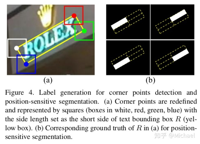
可以看到角点是用矩形代替的，而语义分割图是将矩形分为4个部分来操作的，调用代码是：

target, seg = generate_gt(boxes)

函数generate_gt()为：

def generate_gt(boxes, dim=(512, 512)):
    top_left = []
    top_right = []
    bottom_right = []
    bottom_left = []
    seg = np.zeros((4, dim[0], dim[1]))

    if boxes.size > 0:
        top_left_mask = Image.new('L', (dim[1], dim[0]))
        top_left_draw = ImageDraw.Draw(top_left_mask)
        top_right_mask = Image.new('L', (dim[1], dim[0]))
        top_right_draw = ImageDraw.Draw(top_right_mask)
        bottom_right_mask = Image.new('L', (dim[1], dim[0]))
        bottom_right_draw = ImageDraw.Draw(bottom_right_mask)
        bottom_left_mask = Image.new('L', (dim[1], dim[0]))
        bottom_left_draw = ImageDraw.Draw(bottom_left_mask)
        for i in range(boxes.shape[0]):
            x1, y1, x2, y2, x3, y3, x4, y4 = boxes[i][0], boxes[i][1], boxes[i][2], boxes[i][3], boxes[i][4], boxes[i][5], boxes[i][6], boxes[i][7]
            ## get box
            side1 = math.sqrt(math.pow(x2 - x1, 2) + math.pow(y2 - y1, 2))
            side2 = math.sqrt(math.pow(x3 - x2, 2) + math.pow(y3 - y2, 2))
            side3 = math.sqrt(math.pow(x4 - x3, 2) + math.pow(y4 - y3, 2))
            side4 = math.sqrt(math.pow(x1 - x4, 2) + math.pow(y1 - y4, 2))
            h = min(side1 + side3, side2 + side4)/2.0
            if h*dim[0] >=6:
                theta = math.atan2(y2 - y1, x2 - x1)
                top_left.append(np.array([x1 - h/2, y1 - h/2, x1 + h/2, y1 + h/2, theta, 1]))
                top_right.append(np.array([x2 - h/2, y2 - h/2, x2 + h/2, y2 + h/2, theta, 1]))
                bottom_right.append(np.array([x3 - h/2, y3 - h/2, x3 + h/2, y3 + h/2, theta, 1]))
                bottom_left.append(np.array([x4 - h/2, y4 - h/2, x4 + h/2, y4 + h/2, theta, 1]))
                ## get seg mask
                c1_x, c2_x, c3_x, c4_x, c_x = (x1 + x2)/2.0, (x2 + x3)/2.0, (x3 + x4)/2.0, (x4 + x1)/2.0, (x1 + x2 + x3 + x4)/4.0 
                c1_y, c2_y, c3_y, c4_y, c_y = (y1 + y2)/2.0, (y2 + y3)/2.0, (y3 + y4)/2.0, (y4 + y1)/2.0, (y1 + y2 + y3 + y4)/4.0
                top_left_draw.polygon([x1*dim[1], y1*dim[0], c1_x*dim[1], c1_y*dim[0], c_x*dim[1], c_y*dim[0], c4_x*dim[1], c4_y*dim[0]], fill = 1)
                top_right_draw.polygon([c1_x*dim[1], c1_y*dim[0], x2*dim[1], y2*dim[0], c2_x*dim[1], c2_y*dim[0], c_x*dim[1], c_y*dim[0]], fill = 1)
                bottom_right_draw.polygon([c_x*dim[1], c_y*dim[0], c2_x*dim[1], c2_y*dim[0], x3*dim[1], y3*dim[0], c3_x*dim[1], c3_y*dim[0]], fill = 1)
                bottom_left_draw.polygon([c4_x*dim[1], c4_y*dim[0], c_x*dim[1], c_y*dim[0], c3_x*dim[1], c3_y*dim[0], x4*dim[1], y4*dim[0]], fill = 1)
        seg[0] = top_left_mask
        seg[1] = top_right_mask
        seg[2] = bottom_right_mask
        seg[3] = bottom_left_mask
        if len(top_left) == 0:
            top_left.append(np.array([-1, -1, -1, -1, 0, 0]))
            top_right.append(np.array([-1, -1, -1, -1, 0, 0]))
            bottom_right.append(np.array([-1, -1, -1, -1, 0, 0]))
            bottom_left.append(np.array([-1, -1, -1, -1, 0, 0]))

    else:
        top_left.append(np.array([-1, -1, -1, -1, 0, 0]))
        top_right.append(np.array([-1, -1, -1, -1, 0, 0]))
        bottom_right.append(np.array([-1, -1, -1, -1, 0, 0]))
        bottom_left.append(np.array([-1, -1, -1, -1, 0, 0]))

    top_left = torch.FloatTensor(np.array(top_left))
    top_right = torch.FloatTensor(np.array(top_right))
    bottom_right = torch.FloatTensor(np.array(bottom_right))
    bottom_left = torch.FloatTensor(np.array(bottom_left))

    seg = torch.from_numpy(seg).float()
    seg = seg.permute(1, 2, 0).contiguous()
    return [top_left, top_right, bottom_right, bottom_left], seg

首先会求R的短边，在代码里以h表示，之后就可以根据h和角点坐标得到top_left等四个矩形了。

至于mask，首先生成黑色图像top_left_mask（元素为0），然后生成mask即元素为1的矩形top_left_draw。

4.1.2 Optimization

本节主要讲了loss function：

表示角点检测的概率损失，

表示角点检测的偏差损失，

表示语义分割的损失。

对应的代码为：

loss_l, loss_c, loss_s = criterion(out, targets, segs)
loss_s = loss_s*10
loss = loss_l + loss_c + loss_s

可以看到，10符合论文里

，

的设置。

首先论文给出了

的计算方法：

代码为：

# match priors (default boxes) and ground truth boxes
        loc_t = torch.zeros(num, num_priors, 4, 4).float()
        conf_t = torch.zeros(num, num_priors, 4).long()
        for idx in range(num):
            ## match top_left
            for idx_idx in range(4):
                truths = targets[idx][idx_idx][:, :4].data
                labels = targets[idx][idx_idx][:, -1].data
                defaults = priors.data
                
                match(self.threshold, truths, defaults, self.variance, labels,
                      loc_t, conf_t, idx, idx_idx)

        if self.use_gpu:
            loc_t = loc_t.cuda()
            conf_t = conf_t.cuda()
        # wrap targets
        loc_t = Variable(loc_t, requires_grad=False)
        conf_t = Variable(conf_t, requires_grad=False)

        pos = conf_t > 0
        
        # Localization Loss (Smooth L1)
        # Shape: [batch,num_priors,4]
        pos_idx = pos.unsqueeze(pos.dim()).expand_as(loc_data)
        loc_p = loc_data[pos_idx].view(-1, 4)
        loc_t = loc_t[pos_idx].view(-1, 4)
        loss_l = F.smooth_l1_loss(loc_p, loc_t, size_average=False)

关键是为每一个预测框找出对应的真值框，match()函数里如果jaccard大于0.5就令label为1，否则为0：

Where

is the ground truth of all default boxes, 1 for positive and 0 otherwise.

设置正样本与负样本的比例为1:3：

We use the online hard negative mining proposed in [40] to balance training samples and set the ratio of positives to negetives to 1:3

代码为：

# Compute max conf across batch for hard negative mining
batch_conf = conf_data.view(-1, self.num_classes)

loss_c = log_sum_exp(batch_conf) - batch_conf.gather(1, conf_t.view(-1, 1))

# Hard Negative Mining
loss_c[pos] = 0  # filter out pos boxes for now
loss_c = loss_c.view(num, -1)
_, loss_idx = loss_c.sort(1, descending=True)
_, idx_rank = loss_idx.sort(1)
pos = pos.view(num, -1)
num_pos = pos.long().sum(1, keepdim=True)
num_neg = torch.clamp(self.negpos_ratio*num_pos, max=pos.size(1)-1)
neg = idx_rank < num_neg.expand_as(idx_rank)

控制的参数为self.negpos_ratio，类实例化的时候设置为3。

因此可以得到

的值：

N = num_pos.data.sum()
loss_l /= N

对于偏差损失

，计算为：

代码为：

# Confidence Loss Including Positive and Negative Examples
conf_data_v = conf_data.view(num, -1, self.num_classes)
conf_t_v = conf_t.view(num, -1)

pos_idx = pos.unsqueeze(2).expand_as(conf_data_v)
neg_idx = neg.unsqueeze(2).expand_as(conf_data_v)
conf_p = conf_data_v[(pos_idx+neg_idx).gt(0)].view(-1, self.num_classes)
targets_weighted = conf_t_v[(pos+neg).gt(0)]
        
loss_c = F.cross_entropy(conf_p, targets_weighted, size_average=False)

这里提出一个想法，既然角点矩形是正方形，而Anchor也是正方形，那么三个坐标就可以表示这个offset，注意到论文也是这样表示的，即

。

但是论文却始终在强调有4个offset坐标，比如图3表示的offset branch的公式

中的4就表示有4个offset坐标，个人认为换成3个就满足论文的要求了，而且可以防止4个offset坐标带来的高度和宽度不相等现象，对于这个现象，代码直接将高度舍弃了，我认为这是不太好的一个行为，相关的代码在eval_all.py：

top_left_points.append([(x1 + x2)/2 , (y1 + y2)/2, x2 - x1])

另外一个我认为不好的地方是使用了smooth L1 loss，对一个矩形框来说，位置(y, x)和大小（h, w)对框的作用是不一样的，这里放一张Generalized Intersection over Union: A Metric and A Loss for Bounding Box Regression的图：

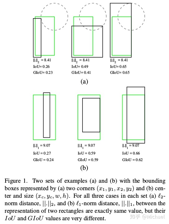
横向对比可以看出，L1距离和L2距离相同的情况IoU和GIoU是不同的。

ps. 直观上可以看出IoU和GIoU更倾向于预测比ground truth box大的矩形框，毕竟

，大的矩形框意味着

增加一个较大的值（

的增加就显得比较迟钝了）。

对于语义分割损失

，公式为：

对应的代码为：

## seg 
eps = 1e-5
seg_gt = segs.view(-1, 1)
intersection = torch.sum(seg_data*seg_gt)
union = torch.sum(seg_data + seg_gt) + eps
loss_s = 1 - 2.0*intersection/union

可以看出，唯有当

且

的时候损失才能为0。

4.2. Inference

4.2.1 Sampling and Grouping

首先需要对角点进行筛选，毕竟网络输出的角点数量过多（确定的说，有120272个），因此，需要根据score过滤、NMS两个步骤：

In inference stage, many corner points are yielded with the predicted location, short side and confidence score. Points with high score (great than 0.5 in default) are kept. After NMS, 4 corner point sets are composed based on relative position information.

对应的代码在layers/functions/detection.py：

for i in range(4):
    decoded_boxes = decode(loc_data[0, :, i, :], prior_data, self.variance)
    conf_scores = conf_preds[0, :, i, :].clone()
    c_mask = conf_scores[:, 1].gt(self.conf_thresh)
    scores = conf_scores[:, 1][c_mask]
    if scores.dim() == 0:
        temp.append(torch.rand(1, 6).fill_(0).cuda())
        continue
    l_mask = c_mask.unsqueeze(1).expand_as(decoded_boxes)
    boxes = decoded_boxes[l_mask].view(-1, 4)
    ids, count = nms(boxes, scores, self.nms_thresh, self.top_k)
    temp.append(torch.cat((scores[ids[:count]].unsqueeze(1),
        boxes[ids[:count]], torch.rand(count, 1).fill_(i).cuda()), 1))

可以看到是分别对四种类型的box进行操作的。

只需要两个角点就可以生成矩形框：

For a predicted point, the short side is known, so we can form a rotated rectangle by sampling and grouping two corner points in corner point sets arbitrarily, such as (top-left, top-right), (top-right, bottom-right), (bottom-left, bottom-right) and (top-left, bottom-left) pairs.

对应的代码是eval_all.py里的get_boxes()函数。

论文还讲了一些生成矩形框的准则，这里就不一一介绍了。

4.2.2 Scoring

与其它文本检测算法不同的是，矩形框的得分并不是直接得到的，而是通过position-sensitive语义分割图得到的：

代码为函数get_score_rpsroi()：

def get_score_rpsroi(bboxes, seg_cuda, rpsroi_pool):
    if len(bboxes) > 0:
        sample_index = torch.zeros(len(bboxes)).view(-1, 1).cuda()
        bboxes = torch.from_numpy(np.array(bboxes)).float().cuda()
        rois = Variable(torch.cat((sample_index, bboxes), 1))
        seg_cuda  = seg_cuda.data
        seg_cuda = torch.index_select(seg_cuda, 1, torch.LongTensor([0, 1, 3, 2]).cuda())
        seg_cuda = Variable(seg_cuda)
        rps_score = rpsroi_pool.forward(seg_cuda, rois)
        return rps_score.data.cpu().view(-1, 4).mean(1).numpy()
    else:
        return np.array([-1])

另外一段代码没有用但我在我本人的项目中用来处理的代码：

def get_score(bbox, seg_pred):
    ## check
    seg_pred = seg_pred.numpy()
    mask = np.zeros(seg_pred.shape)
    c1_x, c2_x, c3_x, c4_x, c_x = (bbox[0] + bbox[2])/2.0, (bbox[2] + bbox[4])/2.0, (bbox[4] + bbox[6])/2.0, (bbox[6] + bbox[0])/2.0, (bbox[0] + bbox[2] + bbox[4] + bbox[6])/4.0
    c1_y, c2_y, c3_y, c4_y, c_y = (bbox[1] + bbox[3])/2.0, (bbox[3] + bbox[5])/2.0, (bbox[5] + bbox[7])/2.0, (bbox[7] + bbox[1])/2.0, (bbox[1] + bbox[3] + bbox[5] + bbox[7])/4.0
    cv2.fillConvexPoly(mask[0], np.array([[bbox[0], bbox[1]*1.0], [c1_x, c1_y], [c_x, c_y], [c4_x, c4_y]]).astype(np.int32), 1)
    cv2.fillConvexPoly(mask[1], np.array([[c1_x, c1_y], [bbox[2]*1.0, bbox[3]*1.0], [c2_x, c2_y], [c_x, c_y]]).astype(np.int32), 1)
    cv2.fillConvexPoly(mask[2], np.array([[c_x, c_y], [c2_x, c2_y], [bbox[4]*1.0, bbox[5]*1.0], [c3_x, c3_y]]).astype(np.int32), 1)
    cv2.fillConvexPoly(mask[3], np.array([[c4_x, c4_y], [c_x, c_y], [c3_x, c3_y], [bbox[6]*1.0, bbox[7]*1.0]]).astype(np.int32), 1)
    score = 0
    for i in range(4):
        score += (mask[i]*seg_pred[i]).sum()/(mask[i].sum())
    score = score/4.0/255.0
    return score

这个代码就与论文的算法1很接近了。

这里说一下这个代码的两个设置：

1.分成

个bins有没有必要。首先，position-sensitive可以对位置比较敏感，看下图也可以发现，如果只有1个bin，如果虚线框得分为1的话，那么小框得分为0.5，两个文本会被合并为一个文本，但是如果有4个bin，虚线框得分为0.25，小框得分则为1，两个文本都被输出；

论文3.3节给出的解释是位置敏感分割的作用是有效地处理相近或相互重叠的文本区域：

However those text regions in score map always can not be separated from each other, as a result of the overlapping of text regions and inaccurate predictions of text pixels.

2.除mask.sum()而不是seg_pred.sum()。这个可以防止框毫无节制的把所有seg数据都包括进去，试想这样的话一个512*512的框得分肯定为1了。但这个也有坏处，就是把文本切小，试想一下，一个文本都向里收缩几个像素，得分依然为1，这个还是很恐怖的；

这里举一个我训练中出现的问题，红框是绿框经过NMS后得到的：

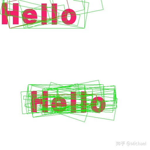
看右下角的文本框，可以看到其实是有更适合hello的文本框的，不过更大，所以score比不上更小的红框（socre为1），这是我认为Corner算法的一个问题了，为了识别的方便，应该宁可把框放的稍微大一些，而不是框放的更小，这样会缺失很多文本信息。

我在网上找了找NMS的改进算法（参考spectre：Detection基础模块之（三）NMS及变体及Soft(er)-NMS：非极大值抑制算法的两个改进算法），但我认为大部分的算法并不符合我的预期：

1. soft NMS抑制分数低的框而不是直接去掉分数低的框，但是我要做的工作是去掉分数高的框（上图的红框），前提不对；
2. softer NMS等附加NMS网络的方法都需要预测框的相关信息，但Corner中的框是后处理工作得到的，直接预测较为复杂；

我的处理思路是不是直接去掉分数低的框，而是去掉分数差大于一定阈值（比如0.2）的框，同时尽可能保留面积大的框。

---

5. Experiments

5.1. Datasets

注意一下各个数据集的侧重点是不一样的，比如ICDAR2013侧重于水平文本检测，MSRA-TD500侧重于多方向文本检测。

5.2.-5.8. Detection Results

注意一下不同的数据集上Corner表现不一样，这跟数据集的分布相关。

水平文本检测Corner甚至低于CTPN和SSTD。

---

6. Conclusion

没啥想讲的。

【已完结】