R pdf大小_数据可视化 - 热图·R-CSDN博客

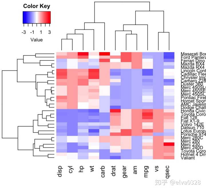
热图（如下图所示），是一种展示样本与差异变量关系的可视化方式，可以通过R/python进行绘制。本文主要分别具体介绍如何使用R实现热图绘制。

R绘制热图

通常调用R的软件包“pheatmap”来进行热图绘制。

# 软件包安装
install.packages("pheatmap")

# 热图绘制
# 先准备好一个数据矩阵matrix.csv，行row为变量，列col为样本。
library('pheatmap')
data=read.table('matrix.csv',sep = ',',stringsAsFactors = F, header =T,row.names = 1)
pdf('heatmap.pdf',height=11,width=12)
pheatmap(as.matrix(data),cluster_cols = F,cluster_rows = F,color = colorRampPalette(colors = c('Blue',"white",'Firebrick1'))(100),annotation_names_row = T)
dev.off()

基本参数用法：

pheatmap(mat, # 数据矩阵
color = colorRampPalette(rev(brewer.pal(n = 7, name = "RdYlBu")))(100), #颜色
kmeans_k = NA, #样本想要聚成几类
breaks = NA, 
border_color = "grey60", #'white' - 热图的每个小块之间以白色隔开
cellwidth = NA, # cell宽度
cellheight = NA, # cell高度，一般选择与cellwidth等长，形成正方形
scale = "none", # 标准化参数，可选"none", "row", "column"
cluster_rows = TRUE,
cluster_cols = TRUE, 
clustering_distance_rows = "euclidean",
clustering_distance_cols = "euclidean", 
clustering_method = "complete",
clustering_callback = identity2, 
cutree_rows = NA, # 根据行的聚类数将热图分隔开
cutree_cols = NA,# 根据列的聚类数将热图分隔开
treeheight_row = ifelse((class(cluster_rows) == "hclust") || cluster_rows,50, 0), 
treeheight_col = ifelse((class(cluster_cols) == "hclust") ||cluster_cols, 50, 0), 
legend = TRUE, legend显示在右上方（可设置legend = FALSE不显示legend）
legend_breaks = NA,
legend_labels = NA, 
annotation_row = NA, 
annotation_col = NA,
annotation = NA, 
annotation_colors = NA, 
annotation_legend = TRUE,
annotation_names_row = TRUE, 
annotation_names_col = TRUE,
drop_levels = TRUE, 
show_rownames = T, 
show_colnames = T, 
main = NA, # main = "热图标题" - 设置热图标题
fontsize = 10, # 字体大小
fontsize_row = fontsize,  # 行字体大小
fontsize_col = fontsize, # 列字体大小
angle_col = c("270", "0", "45", "90", "315"), 
display_numbers = F,
number_format = "%.2f", 
number_color = "grey30", 
fontsize_number = 0.8 * fontsize, 
gaps_row = NULL, # 设定行要分隔开的位置 gaps_row = c(10, 14)
gaps_col = NULL, # 设定列要分隔开的位置 cutree_col = 2
labels_row = NULL,
labels_col = NULL, 
filename = NA, # "result.pdf"
width = NA, 
height = NA,
silent = FALSE, 
na_col = "#DDDDDD", 
...)

其中pheatmap的主要参数如下：

pheatmap(as.matrix(data),cluster_cols = F,cluster_rows = F,color = colorRampPalette(colors = c('Blue',"white",'Firebrick1'))(100),annotation_names_row = T)

# cluster - 进行聚类（可设置cluster_row = FALSE, cluster_col = FALSE不进行行列的聚类）
# 如果进行聚类了，还可以通过设置treeheight_row=0, treeheight_col=0不显示dendrogram
# scale - 标准化参数，可选"none", "row", "column"
# border_color = 'white' - 热图的每个小块之间以白色隔开
# 如果不想要border可以设置为NA，当然也可以设置成其它颜色
# legend显示在右上方（可设置legend = FALSE不显示legend）
# cellwidth - cell宽度
# cellheight  - cell高度，一般选择与cellwidth等长，形成正方形
# main = "热图标题" - 设置热图标题
# fontsize - 字体大小
# filename = "result.pdf"

如果有样本分类信息，还可以加上分类bar：

annotation_col = data.frame(CellType = factor(rep(c("CT1", "CT2"), 5)))
# 不均衡的分类 - CellType = factor(rep(c("CT1", "CT2"), c(4, 6)))
rownames(annotation_col) <- colnames(data) #分类和样本名称对应

如果有变量分类信息，还可以加上变量分类bar：

annotation_row = data.frame(GeneClass = factor(rep(c("Path1", "Path2", "Path3"), c(10, 4, 6))))
rownames(annotation_row) = rownames(data)

分类bar的颜色标注：

ann_colors = list(CellType = c(CT1 = "#1B9E77", CT2 = "#D95F02"),
GeneClass = c(Path1 = "#7570B3", Path2 = "#E7298A", Path3 = "#66A61E"),
Time = c("white", "firebrick") #连续数值型分组可设置成渐变）

pheatmap(data, annotation_col = annotation_col, annotation_row = annotation_row,
         annotation_colors = ann_colors)

# annotation_legend=TRUE - 显示样本分类
# show_rownames = T - 显示行名
# show_colnames = T - 显示列名
# color =colorRampPalette(c("#3B8194", "#ffffff","#E50031"))(100) - 热图基准颜色

参考资料：

https://www.rdocumentation.org/packages/pheatmap/versions/1.0.12/topics/pheatmap
pheatmap