


语句 with ... as ... :
在Python2.6以后版本引入了 with 语句,如以下代码
with open("myfile", "r") as f:

    print f.readline()
其等价语句是
f = file("myfile", "r")
try:
    print f.readline()
execpt Exception:
    pass
finally:
f.close()一对比发现,with语言显得更加简洁,原因就是open对象实现了上下文管理协议(context manage), 既在class中实现了 __enter__ 和 __exit__ 两个方法,如果要自己实现一个支持上下文协议的对象,那么在这个对象中必须实现这两个方法。此案例来自<Python中with的介绍以及高级用法>,其文中还有错误调试等内容未看.
np.asarray()和np.array()区别
array和asarray都可以将结构数据转化为ndarray,但是主要区别就是当数据源是ndarray nameA时,array仍然会copy出一个副本nameB,占用新的内存,nameA和nameB是脱钩的。但asarray不会,asarray生成的数组nameC和nameA挂钩,对nameC和nameA的操作是互相关联的。
A = numpy.matrix(np.ones((3,3)))
>>> A  matrix([[ 1., 1., 1.], [ 1., 1., 1.], [ 1., 1., 1.]])
# 使用numpy.array修改A。由于修改的是副本,而不是源数组A,而不起作用
numpy.array(A)[2] = 2
>>> A  matrix([[ 1., 1., 1.], [ 1., 1., 1.], [ 1., 1., 1.]])
# 使用numpy.asarray修改A则有用,因为修改A本身
numpy.asarray(A)[2]=2
>>> A  matrix([[ 1., 1., 1.], [ 1., 1., 1.], [ 2., 2., 2.]])
# example 2:
arr1=np.ones((3,3))
arr2=np.array(arr1)
arr3=np.asarray(arr1)
arr1[1]=2
print ('arr1:n',arr1)
print ('arr2:n',arr2)
print ('arr3:n',arr3)
# 输出:
rr1: [[ 1.  1.  1.] [ 2.  2.  2.] [ 1.  1.  1.]]
arr2:[[ 1.  1.  1.] [ 1.  1.  1.] [ 1.  1.  1.]]
arr3:[[ 1.  1.  1.] [ 2.  2.  2.] [ 1.  1.  1.]]
np.mean(arr)和np.var(arr)和np.std(arr,ddof=1)
Python求均值,方差,标准差。注意:
- np.std()求标准差和np.var()求方差时,缺省ddof=0, 求总体标准差/方差,默认是除以 n 的,即是有偏的;若要求无偏的 样本标准差/方差,即除以n-1,需设置参数 ddof = 1;
- pandas.std() 相反,默认是除以n-1 的,即是无偏的,如果想和numpy.std() 一样有偏,需要加上参数ddof=0 ,即pandas.std(ddof=0) ;DataFrame的describe()中就包含有std();(是说pandas.std?)
- 关于总体方差和样本方差之区别、原因参见我的帖子<补充附录(9)数据处理相关:样本方差和总体方差>
import numpy as np
a = np.array([0, 1, 2, 3, 4, 5, 6, 7, 8, 9])
print("------缺省-------")
print("平均值为:%f" % np.mean(a))
print("方差为:%f" % np.var(a))
print("标准差为:%f" % np.std(a))
print("------非缺省-------")
print(np.std(a, ddof = 1))
print(np.sqrt(((a - np.mean(a)) ** 2).sum() / (a.size - 1)))
print(np.sqrt(( a.var() * a.size) / (a.size - 1)))
------缺省-------
平均值为:4.500000
方差为:8.250000
标准差为:2.872281
------非缺省-------
3.0276503540974917
3.0276503540974917
3.0276503540974917
tf.shape()
import tensorflow as tf
A=[[1,2,3],
   [4,5,6]]
t = tf.shape(A)

with tf.Session() as sess:
    print(sess.run(t))

out: [2 3]
np.reshape(x,[-1,28,28,1])中某一维度=-1的含义
重新排列x,其他维度数目给定,该维度数目相应自动计算得到
z = np.array([[1, 2, 3, 4],
          [5, 6, 7, 8],
          [9, 10, 11, 12],
          [13, 14, 15, 16]])
z.shape
(4, 4)
z.reshape(-1)
z.reshape(-1)
array([ 1,  2,  3,  4,  5,  6,  7,  8,  9, 10, 11, 12, 13, 14, 15, 16])
z.reshape(-1, 1)
也就是说,先前我们不知道z的shape属性是多少,但是想让z变成只有一列,行数不知道多少,通过`z.reshape(-1,1)`,Numpy自动计算出有16行,新的数组shape属性为(16, 1),与原来的(4, 4)配套。注意reshape(-1, 1)和reshape(-1)的区别,本质上是(n,)和(n,1)的区别。
z.reshape(-1,1)
 array([[ 1],
        [ 2],
        [ 3],
        [ 4],
        [ 5],
        [ 6],
        [ 7],
        [ 8],
        [ 9],
        [10],
        [11],
        [12],
        [13],
        [14],
        [15],
        [16]])
z.reshape(-1, 2)
newshape等于-1,列数等于2,行数未知,reshape后的shape等于(8, 2)
z.reshape(-1, 2)
 array([[ 1,  2],
        [ 3,  4],
        [ 5,  6],
        [ 7,  8],
        [ 9, 10],
        [11, 12],
        [13, 14],
        [15, 16]])
同理,只给定行数,newshape等于-1,Numpy也可以自动计算出新数组的列数。其他维度也是一样。
enumerate()
python的内置函数,多用于在for循环中得到计数。对于一个可迭代的(iterable)/可遍历的对象(如列表、字符串),enumerate将其组成一个索引序列,利用它可以同时获得索引和值
(1)如果对一个列表,既要遍历索引又要遍历元素时,首先可以这样写:
list1 = ["这", "是", "一个", "测试"]
for i in range (len(list1)):
    print i ,list1[i]
(2)上述方法有些累赘,利用enumerate()会更加直接和优美:
list1 = ["这", "是", "一个", "测试"]
for index, item in enumerate(list1):
    print index, item
>>>
0 这
1 是
2 一个
3 测试
(3)enumerate还可以接收第二个参数,用于指定索引起始值,如:
list1 = ["这", "是", "一个", "测试"]
for index, item in enumerate(list1, 1):
    print index, item
>>>
1 这
2 是
3 一个
4 测试
(4)如果要统计文件的行数,可以这样写:
count = len(open(filepath, 'r').readlines())
这种方法简单,但是可能比较慢,当文件比较大时甚至不能工作。
(5)此时, 可以利用enumerate():
count = 0
for index, line in enumerate(open(filepath,'r')):
    count += 1
tf.concat, tf.stack和tf.unstack的用法
tf.concat相当于numpy中的np.concatenate函数,用于将两个张量在某一个维度(axis)合并起来,例如:
a = tf.constant([[1,2,3],[3,4,5]]) # shape (2,3)
b = tf.constant([[7,8,9],[10,11,12]]) # shape (2,3)
ab1 = tf.concat([a,b], axis=0) # shape(4,3)
ab2 = tf.concat([a,b], axis=1) # shape(2,6)tf.stack其作用类似于tf.concat,都是拼接两个张量,而不同之处在于,tf.concat拼接的是除了拼接维度axis外其他维度的shape完全相同的张量,并且产生的张量的阶数不会发生变化,而tf.stack则会在新的张量阶上拼接,产生的张量的阶数将会增加,例如:
a = tf.constant([[1,2,3],[3,4,5]]) # shape (2,3)
b = tf.constant([[7,8,9],[10,11,12]]) # shape (2,3)
ab = tf.stack([a,b], axis=0) # shape (2,2,3)
axis是决定其层叠(stack)张量的维度方向的,改变参数axis为2,有:
import tensorflow as tf
a = tf.constant([[1,2,3],[3,4,5]]) # shape (2,3)
b = tf.constant([[7,8,9],[10,11,12]]) # shape (2,3)
ab = tf.stack([a,b], axis=2) # shape (2,3,2)
abc = tf.stack([a,b], axis=1) # shape (2,3,2)
# 这个按行和列拼接成更高维的方法,也是很迷了。用羊肉串思考法,比较不错 hahahaha而tf.unstack与tf.stack的操作相反,是将一个高阶数的张量在某个axis上分解为低阶数的张量,例如:
a = tf.constant([[1,2,3],[3,4,5]]) # shape (2,3)
b = tf.constant([[7,8,9],[10,11,12]]) # shape (2,3)
ab = tf.stack([a,b], axis=0) # shape (2,2,3)
a1 = tf.unstack(ab, axis=0)
# 输出 [<tf.Tensor 'unstack_1:0' shape=(2,3) dtype=int32>,
<tf.Tensor 'unstack_1:1' shape=(2,3) dtype=int32>]
np.random.shuffle()
shuffle()的作用是混排序列中的元素,序列中元素顺序改变,但其内容不变. 多维数组则只改变第一个轴的元素顺序,如对2维张量,各行向量相对位置会混排。shuffle这个概念会在多处出现,混排核心思想是一致的
import numpy as np
a = np.arange(10)
print("a=", a )
np.random.shuffle(a)
print("After shuffle, a=", a )

a= [0 1 2 3 4 5 6 7 8 9]
After shuffle, a= [8 1 6 4 2 7 0 9 3 5]
tf.less()
返回两个张量各元素比较(x<y)得到的真假值组成的张量
import tensorflow as tf
A=[[1,2,3],
   [4,5,6]]
t = tf.shape(A)
i=[[1,2,3],
   [1,2,3]]
r = tf.less(i, A)
with tf.Session() as sess:
    print(sess.run(t))
    print(sess.run(r))

out:[2 3]
[[False False False]
 [ True  True  True]]
tf.greater()
输入时两个张量,这个函数会比较两个输入张量中每一个元素的大小,然后返回一个bool类型的tensor,如果两个张量的维度不一致的话,会报错。
import tensorflow as tf
A=[[1,2,3],
   [4,5,6]]
temp=[[2,3],
      [5,6]]
i=[[1,2,3],
   [1,2,3]]

#r1 = tf.greater(temp, A)  # 报错
r2 = tf.greater(i, A)
with tf.Session() as sess:
   # print(sess.run(r1))
    print(sess.run(r2))

out: [[False False False]
 [False False False]]
tf.equal(A, B)
输入两个维度相同的张量(数据类型似乎不必相同),比较这两个张量中各位置处元素是否相等,如果是相等的则返回True,不相等则返回False,返回的值的张量,其维度和A是一样的。
import tensorflow as tf
A = [[1.1,3.1,4.1,5.1,6.0]]  # 浮点型。但若维度不一样,则会报错
B = [[1,3,4,3,4]]            # 整形
with tf.Session() as sess:
    print(sess.run(tf.equal(A, B)))

out: [[False False False False False]]
tf.where()
函数有三个参数,根据第一个条件是否成立,当为True的时候选择第二个参数中的值,否则使用第三个参数中的值。示例如下
loss = tf.reduce_sum (tf.where(tf.greater(v1,v2), (v1 - v2 ) * a, (v2 -v1) * b))tf.argmax(tensor, 1)
返回的是tensor中的每一行中最大值的索引号 组成的数组,该数组比输入tensor降了一个维度。输入tensor至少是2维.(二维是这样的,但三维及以上,不知道这个返回值是怎么得来的,如下??在琢磨一下)
A0 = [1,3,4,5,6]
A = [[1,3,4,5,6]]
B = [[1,3,4], [2,4,1]]
C= [[1,2],[19,9],[3,5]]
D = [[[1,2],[19,9]],[[3,5],[11,14]]]
with tf.Session() as sess:
   # print(sess.run(tf.argmax(A0, 1))) # 会报错
   print(sess.run(tf.argmax(A, 1)))
   print(sess.run(tf.argmax(B, 1)))
   print(sess.run(tf.argmax(C, 1)))
   print(sess.run(tf.argmax(D, 1)))

out:
[4]  # A中第一行最大值6索引号为4.第一个位置索引为0
[2 1]
[1 0 1]
[[1 1]
 [1 1]]
tf.assign(A, new_number)
函数功能主要是把A的值变为new_number
import tensorflow as tf;
A = tf.Variable(tf.constant(0.0), dtype=tf.float32)
with tf.Session() as sess:
	sess.run(tf.initialize_all_variables())
	print sess.run(A)
	sess.run(tf.assign(A, 10))

out: 0.0
10.0
zip(x,y)
注意无需tf. 前缀。将不同对象中相对应的元素打包成一个元组(tuple),返回由这些元组组成的list列表,如果传入的参数的长度不等,则返回的list列表的长度和传入参数中最短对象的长度相同。
a = [1,2,3,4,5]
b = ['a','b','c','d']
c = [[1,2,3,4],['a','b','c'],[7,8,9]]
x1 = zip(a,b)
x2 = zip(a)
x3 = zip(*c)  # 行之间zip,降维

out:
x1 = [(1, 'a'), (2, 'b'), (3, 'c'), (4, 'd')]
x2 = [(1,), (2,), (3,), (4,), (5,)]
x3 = [(1, 'a', 7), (2, 'b', 8), (3, 'c', 9)]
tf.multiply(x, y, name=None)
- element-wise相乘,x,y可以为矩阵,也可为数,一维向量。不是矩阵乘法,区别tf.matmul
- x和y必须有相同的数据类型,不然就会报错. 数据类型可选half(即float16), float32, float64, uint8, int8, uint16, int16, int32, int64, complex64, complex128
tf.matmul(a, b, transpose_a=False, transpose_b=False, adjoint_a=False, adjoint_b=False, a_is_sparse=False, b_is_sparse=False, name=None)
- 矩阵相乘,输入a和b需为矩阵(不能是数和一维向量),必须为相同数据类型,可选同上
- transpose/adjoint/sparse表示计算前是否进行转置/共轭和转置/被处理为稀疏矩阵
import tensorflow as tf
#两个矩阵的对应元素各自相乘!!
x=tf.constant([[1.0,2.0,3.0],[1.0,2.0,3.0],[1.0,2.0,3.0]])
# 其实x=tf.constant([[1,2,3.0],[1.0,2.0,3.0],[1.0,2.0,3.0]])也是对的,有一个浮点型就把全部带成浮点型了
y=tf.constant([[0,0,1.0],[0,0,1.0],[0,0,1.0]])
#注意这里这里x,y要有相同的数据类型,不然就会因为数据类型不匹配而出错
z=tf.multiply(x,y)

#两个数相乘
x1=tf.constant(1)
y1=tf.constant(2)
#注意这里这里x1,y1要有相同的数据类型,不然就会因为数据类型不匹配而出错
z1=tf.multiply(x1,y1)

#数和矩阵相乘
x2=tf.constant([[1.0,2.0,3.0],[1.0,2.0,3.0],[1.0,2.0,3.0]])
y2=tf.constant(2.0)
#注意这里这里x2,y2要有相同的数据类型,不然就会因为数据类型不匹配而出错
z2=tf.multiply(x2,y2)

#两个矩阵相乘
x3=tf.constant([[1.0,2.0,3.0],[1.0,2.0,3.0],[1.0,2.0,3.0]])
y3=tf.constant([[0,0,1.0],[0,0,1.0],[0,0,1.0]])
#注意这里这里x,y要满足矩阵相乘的格式要求。
z3=tf.matmul(x,y)

输出为
[[0. 0. 3.]
 [0. 0. 3.]
 [0. 0. 3.]]
2
[[2. 4. 6.]
 [2. 4. 6.]
 [2. 4. 6.]]
[[0. 0. 6.]
 [0. 0. 6.]
 [0. 0. 6.]]
tf.math.subtract(x, y, name=None) 或 tf.subtract(x, y, name=None)
- 返回与被减数张量具有相同类型的张量,可以为矩阵-数
- 旧版本的tf.sub()已被废弃
矩阵加减法
根据张量加法规则,(m,n)张量可以和(n,1)张量相加,效果就是(m,n)中每一行都和(n,1)相加
例如,[[0,0,0],[0,0,0]]+[1,2,3]=[[1,2,3],[1,2,3]]。减法也是类似的,不知道为什么这么规定。
tf.nn.softmax()
通过Softmax回归,将logistic的预测二分类的概率的问题推广到了n分类的概率的问题。通过公式
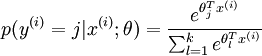
可以看出当月分类的个数变为2时,Softmax回归又退化为logistic回归问题。
A = tf.constant([[1.0,2.0,3.0],[1.0,2.0,3.0],[1.0,2.0,3.0]])
with tf.Session() as sess:
     print(sess.run(tf.nn.softmax(A)))
# 输出
[[0.09003057 0.24472848 0.66524094]
 [0.09003057 0.24472848 0.66524094]
 [0.09003057 0.24472848 0.66524094]]
其中每一行所有输出的和为1.
tf.nn.softmax_cross_entropy_with_logits(logits, labels, name=None)
用于逻辑回归。第一个参数logits为神经网络最后一层的输出,如果有batch的话,它的大小就是[batchsize,num_classes],单样本的话,大小就是num_classes。第二个参数labels为实际的标签。
输入logits是前一层网络做一个softmax的输出,这一步通常是求取输出属于某一类的概率,对于单样本而言,输出就是一个num_classes大小的向量([Y1,Y2,Y3...Y10]其中Y1,Y2,Y3...分别代表了是属于该类的概率,例如mnist数据集某张图片,训练得到[0.1, 0.9, 0,0,0.....0])。softmax的公式如上所述。
本公式输出是logits, labels做的一个交叉熵,公式为
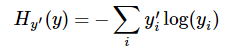
其中
tf.reduce_mean操作,对N个样本所对应的N个
import tensorflow as tf
train_data=tf.constant([[1.0,2.0,3.0],[1.0,2.0,3.0],[1.0,2.0,3.0]])
y_hat=tf.nn.softmax(train_data)
#true label
y_label=tf.constant([[1.0,0.0,0.0],[0.0,1.0,0.0],[1.0,0.0,0.0]])
cross_entropy=tf.nn.softmax_cross_entropy_with_logits(labels=y_label,logits=y_hat)
# 计算3个样本的平均loss
avg_loss = tf.reduce_mean(cross_entropy)
with tf.Session() as sess:
    print(sess.run(y_hat))
    print(sess.run(cross_entropy))
    print(sess.run(avg_loss))
>>> [[0.09003057 0.24472848 0.66524094]
 [0.09003057 0.24472848 0.66524094]
 [0.09003057 0.24472848 0.66524094]]
>>> [1.3724008 1.2177029 1.3724008]
>>> 1.3208348
奇怪:手动计算y_hat得到结果和这里一致,例如e^1/(e^1+e^2+e^3)=0.09003057。但是计算交叉熵得不到上面的结果呀log(0.09003057)≠1.3724008 啊,不知道计算机怎么得到的??奇怪
tf.variable_scope()和tf.name_scope()限定变量作用域
TF中有两种作用域类型:命名域(name scope),通过tf.name_scope 或 tf.op_scope创建;变量域(variable scope),通过tf.variable_scope 或 tf.variable_op_scope创建;作用域函数tf.name_scope()、tf.variable_scope()一般与两个创建/调用变量的函数tf.variable() 和tf.get_variable()搭配使用,作用是1)设定的作用域范围内进行变量共享;2)tensorboard画流程图进行可视化封装变量。
- tf.variable_scope 允许利用tf.get_variable使用已经创建的变量,允许利用tf.Variable创建新变量
- tf.name_scope 只允许利用tf.Variable创建新变量
- 根据reuse=(True, False, tf.AUTO_REUSE), 'V1'名称,是tf.get_variable还是tf.Variable,是tf.variable_scope还是tf.name_scope,最后形成V1/a1:0, V1/a11:0, V1/a1_2:0, V1_1/a1:0等结果。注意tf.variable_scope('V1')接着tf.name_scope('V1'),则会形成V1_1。如果连续用同类函数名称,则不会出现V1_1。参加下面例子
更多内容参见<tf.variable_scope和tf.name_scope的用法><通俗理解tf.name_scope()、tf.variable_scope()>
import tensorflow as tf
import numpy as np
import matplotlib.pyplot as plt

with tf.variable_scope('V1',reuse=tf.AUTO_REUSE):
    a1 = tf.get_variable(name='a1', shape=[1], initializer=tf.constant_initializer(1))
    a2 = tf.Variable(tf.random_normal(shape=[2,3], mean=0, stddev=1), name='a2')
    a3 = tf.get_variable(name='a1', shape=[1], initializer=tf.constant_initializer(1))
    a4 = tf.Variable(tf.random_normal(shape=[2,3], mean=0, stddev=1), name='a1')
    a5 = tf.get_variable(name='a2', shape=[1], initializer=tf.constant_initializer(1))
with tf.variable_scope('V2'):
    a6 = tf.get_variable(name='a1', shape=[1], initializer=tf.constant_initializer(1))
    a7 = tf.Variable(tf.random_normal(shape=[2,3], mean=0, stddev=1), name='a2')
with tf.variable_scope('V1',reuse=False):
    # 会报错,因为可重用设置为否
    # a8 = tf.get_variable(name='a1', shape=[1], initializer=tf.constant_initializer(1))
    a9 = tf.Variable(tf.random_normal(shape=[2,3], mean=0, stddev=1), name='a2')

with tf.Session() as sess:
    sess.run(tf.initialize_all_variables())
    print('a1=',a1.name)
    print('a2=',a2.name)
    print('a3=',a3.name)
    print('a4=',a4.name)
    print('a5=',a5.name)
    print('a6=',a6.name)
    print('a7=',a7.name)
    print('a8=',a6.name)
    print('a9=',a7.name)
输出:
a1= V1/a1:0
a2= V1/a2:0
a3= V1/a1:0
a4= V1/a1_1:0
a5= V1/a2_1:0
a6= V2/a1:0
a7= V2/a2:0
a8= V2/a1:0
a9= V2/a2:0

with tf.name_scope('V1'):
    # 下面这行会报错
    # a1 = tf.get_variable(name='a1', shape=[1], initializer=tf.constant_initializer(1))
    a2 = tf.Variable(tf.random_normal(shape=[2,3], mean=0, stddev=1), name='a2')
with tf.name_scope('V2'):
    # a3 = tf.get_variable(name='a1', shape=[1], initializer=tf.constant_initializer(1))
    a4 = tf.Variable(tf.random_normal(shape=[2,3], mean=0, stddev=1), name='a2')

with tf.Session() as sess:
    sess.run(tf.initialize_all_variables())
    # print('a1=',a1.name)
    print('a2=',a2.name)
    # print('a3=',a3.name)
    print('a4=',a4.name)
输出:
a2= V1_1/a2:0
a4= V2_1/a2:0
np.c_[] 和 np.r_[]
- np.r_是指可变动row行数,保持列数不变,按列连接两个矩阵,要求列数相等,类似于pandas中的concat()。
- np.c_是指可变动clolumn列数,保持行数不变,按行连接两个矩阵,要求行数相等,类似于pandas中的merge()。
- 注意是[],不是()小括号。会报错,已验证
- 注意一维张量是列向量/列矩阵,n行1列。下面第一个例子可见
import numpy as np
a = np.array([1, 2, 3])
b = np.array([4, 5, 6])
c = np.c_[a,b]
a1 = np.array([[1, 2, 3],[4,5,6]])
b1 = np.array([[0, 0, 0],[1,1,1]])

print(np.r_[a,b])
print(c)
print(np.c_[c,a])
print(np.r_[a1,b1])
print(np.c_[a1,b1])
输出:
[1 2 3 4 5 6]

[[1 4]
 [2 5]
 [3 6]]

[[1 4 1]
 [2 5 2]
 [3 6 3]]

[[1 2 3]
[4 5 6]
[0 0 0]
[1 1 1]]

[[1 2 3 0 0 0]
[4 5 6 1 1 1]]


 被折叠的 条评论
为什么被折叠?
被折叠的 条评论
为什么被折叠?
 到【灌水乐园】发言


