使用预训练的VGG16卷积基作特征提取

前言

将深度学习用于小型图像数据集，一种常用且高效的方法是使用预训练的网络。预训练网络是一个在大型数据集上训练好的模型，因为训练数据集足够大，使的该模型学到的特征的空间层次结构可以有效地作为视觉世界的通用模型，所以可以将这些特征用于各种不同的计算机视觉任务，即使新问题涉及的类别和原始任务完全不同。
使用预训练网络有两种方法：1、特征提取；2、微调模型。
本文主要阐述第一种方法。

一、VGG16模型权重下载

from keras.applications import VGG16

conv_base = VGG16(weights='imagenet',
                  include_top=False,
                  input_shape=(150, 150, 3)
                  )

说明： 用以上代码默认下载VGG16权重文件的地址是：
https://github.com/fchollet/deep-learning-models/releases/download/v0.1/vgg16_weights_tf_dim_ordering_tf_kernels_notop.h5
在谷歌浏览器下网页不能打开。
因此，在网页搜索手动下载，我这里的下载地址为百度云：
https://pan.baidu.com/s/16IXUTp1brcYqkSi_A0u55A
提取码：8487
下载下来是一个vgg16.npy文件，553M大小。

二、VGG16权重加载和保存

import numpy as np
from keras.applications import VGG16

data_dict=np.load('./vgg16.npy',encoding='latin1',allow_pickle=True).item()  # vgg16.npy在当前目录下存放
model= VGG16(weights=None,include_top=False)   # 不包括密集连接分类器部分
model.layers[1].set_weights(data_dict['conv1_1'])
model.layers[2].set_weights(data_dict['conv1_2'])
model.layers[4].set_weights(data_dict['conv2_1'])
model.layers[5].set_weights(data_dict['conv2_2'])
model.layers[7].set_weights(data_dict['conv3_1'])
model.layers[8].set_weights(data_dict['conv3_2'])
model.layers[9].set_weights(data_dict['conv3_3'])
model.layers[11].set_weights(data_dict['conv4_1'])
model.layers[12].set_weights(data_dict['conv4_2'])
model.layers[13].set_weights(data_dict['conv4_3'])
model.layers[15].set_weights(data_dict['conv5_1'])
model.layers[16].set_weights(data_dict['conv5_2'])
model.layers[17].set_weights(data_dict['conv5_3'])

model.save("VGG16.h5")
model.save_weights("VGG16_weights.h5")   # 保存模型在当前目录下

三、使用VGG16卷积基提取特征

from keras.applications import VGG16
import os
import numpy as np
from keras.preprocessing.image import ImageDataGenerator

conv_base = VGG16(weights='./VGG16_weights.h5',       # 加在保存的权重文件
                  include_top=False,
                  input_shape=(150, 150, 3)
                  )
base_dir = "./dogs_and_cats_small"
train_dir = os.path.join(base_dir, 'train')
validation_dir = os.path.join(base_dir, 'validation')
test_dir = os.path.join(base_dir, 'test')                  

datagen = ImageDataGenerator(rescale=1./255)
batch_size=20

## TODO 使用预训练卷积提取特征
def extract_features(directory, sample_count):
    features = np.zeros(shape=(sample_count, 4, 4, 512))
    labels = np.zeros(shape=(sample_count))

    generator = datagen.flow_from_directory(
        directory,
        target_size=(150, 150),
        batch_size=batch_size,
        class_mode='binary'
    )
    i = 0
    for input_batch, labels_batch in generator:
        features_batch = conv_base.predict(input_batch)                    # 提取特征
        features[i*batch_size:(i+1)*batch_size] = features_batch
        labels[i*batch_size:(i+1)*batch_size] = labels_batch
        i += 1
        if i*batch_size >=sample_count:
            break
    return features, labels

train_features, train_labels = extract_features(train_dir, 2000)
validation_features, validation_labels = extract_features(validation_dir, 1000)
test_features, test_labels = extract_features(test_dir, 1000)

train_features = np.reshape(train_features, (2000, 4*4*512))
validation_features = np.reshape(validation_features, (1000, 4*4*512))
test_features = np.reshape(test_features, (1000, 4*4*512))

四、自定义和训练密集连接分类器

from keras import models
from keras import layers
from keras import optimizers
import matplotlib.pyplot as plt

model = models.Sequential()
model.add(layers.Dense(256, activation='relu', input_dim=4*4*512))
model.add(layers.Dropout(0.5))
model.add(layers.Dense(1, activation='sigmoid'))

model.compile(optimizer=optimizers.RMSprop(lr=2e-5),
              loss='binary_crossentropy',
              metrics=['acc'])

history = model.fit(train_features, train_labels, epochs=30, batch_size=20, 
                    validation_data=(validation_features, validation_labels))

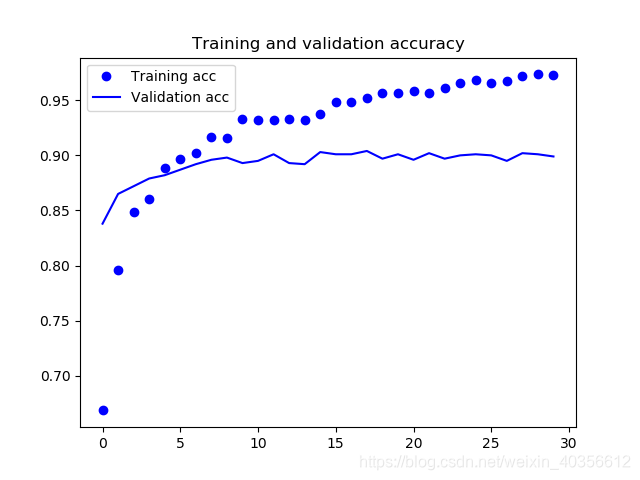
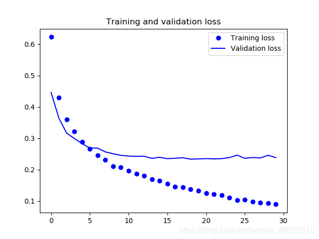
五、绘制训练和验证精度和损失曲线

acc = history.history['acc']
val_acc = history.history['val_acc']
loss = history.history['loss']
val_loss = history.history['val_loss']

epochs = range(len(acc))

plt.plot(epochs, acc, 'bo', label='Training acc')
plt.plot(epochs, val_acc, 'b', label = 'Validation acc')
plt.title("Training and validation accuracy")
plt.legend()

plt.figure()

plt.plot(epochs, loss, 'bo', label='Training loss')
plt.plot(epochs, val_loss, 'b', label='Validation loss')
plt.title("Training and validation loss")
plt.legend()

plt.show()

训练和验证精度曲线

训练和验证损失曲线

六、结论

训练精度几乎达到90%了。

参考文献

• https://blog.csdn.net/weixin_44621626/article/details/105028109
• 佛朗索瓦.肖莱著，张亮译. Python深度学习[M]. 人民邮电出版社.2018.8.p116-121.

END