cartographer_learn_13点云匹配

续接上篇

第12篇，点云匹配前的数据处理
本来估计怎么的也得一周才会更新的，没想到ceres的使用（仅仅是使用）比作者想象的简单一点。没有像学g2o的时候有一些当时看起来比较奇怪的概念（一元边（第一次接触时在想一个顶点怎么能画边呢？。。。。。。））。好了回忆一下第12篇中点云处理的结果，最终我们得到的点云是在tracking坐标系下点p乘以一个旋转（imu数据估计出来的tracking坐标系的旋转），且这里所说的tracking坐标系时对应点云中最后一个点的时间的tracking坐标系。在说匹配前还有一些步骤我们没有讨论过，比如自适应体素滤波和地图究竟是什么样的。我们接下来一点点来学习。

匹配前剩余的一些操作

先看看在前端中最顶层的调用，

std::unique_ptr<LocalTrajectoryBuilder2D::MatchingResult>
LocalTrajectoryBuilder2D::AddRangeData(
    const std::string& sensor_id,
    const sensor::TimedPointCloudData& unsynchronized_data) {
......//多个传感器数据打包
......//位姿推断器初始化
......//一些检查
......//功能1
......//功能2
//看到并不是每次分发LaserScan的数据后都做匹配，而是等待一定次数后才做匹配
if (......) {
    .......//一些其他的操作，第12篇有介绍
    return AddAccumulatedRangeData(
        time,
        // 对点云做处理，体素滤波
        TransformToGravityAlignedFrameAndFilter(
            gravity_alignment.cast<float>() * range_data_poses.back().inverse(),
            accumulated_range_data_),
        gravity_alignment, sensor_duration);
  }
  return nullptr;
}

这里我们主要去看看LocalTrajectoryBuilder2D::AddAccumulatedRangeData这个方法，上代码：

std::unique_ptr<LocalTrajectoryBuilder2D::MatchingResult>
LocalTrajectoryBuilder2D::AddAccumulatedRangeData(
    const common::Time time,
    const sensor::RangeData& gravity_aligned_range_data,
    const transform::Rigid3d& gravity_alignment,
    const absl::optional<common::Duration>& sensor_duration) {
  if (gravity_aligned_range_data.returns.empty()) {
    LOG(WARNING) << "Dropped empty horizontal range data.";
    return nullptr;
  }

  // 给出tracking坐标系位姿的初值
  const transform::Rigid3d non_gravity_aligned_pose_prediction =
      extrapolator_->ExtrapolatePose(time);
  //这里可以直接告诉读者，匹配得到的结果并不是tracking坐标的位姿，而是这个矩阵（虽然不是矩阵形式表示），
  //同样的不要试图去理解这个举证的物理意义，因为它就是个中间量，没有特别明确的物理意义
  const transform::Rigid2d pose_prediction = transform::Project2D(
      non_gravity_aligned_pose_prediction * gravity_alignment.inverse());
  //自适应体素滤波
  const sensor::PointCloud& filtered_gravity_aligned_point_cloud =
      sensor::AdaptiveVoxelFilter(gravity_aligned_range_data.returns,
                                  options_.adaptive_voxel_filter_options());
  if (filtered_gravity_aligned_point_cloud.empty()) {
    return nullptr;
  }
  .......//一些其他的操作
}

这里像串联一下思路，第12篇得到的点云可以如公式1这样表示（注意这里的tracking坐标系对应的时间）

如果我们直接拿tracking坐标系位姿做匹配，那将无法把点转换到local坐标系中，所以我们要使用上诉代码中的那个矩阵作为转换转换矩阵参与匹配，最后再把结果转换回来。

自适应体素滤波

先提醒读者注意看体素滤波的第一个实参，只使用了returnes，忽略了misses，所以即使我们不太理解为什么要那样操作misses中的点也没关系，因为它在后面（至少再匹配中）没有使用。
作者把自适应体素滤波的源码看下来，认为它的目的就在与保证每次参与匹配的点云中的点的数量都差不多，在某个数的附近，这样做是为了确保每次处理的速度和结果精度的一致性。同时在自适应体素 滤波前还有一个函数，虽然使用了lambda表达式，但其功能很简单（去除掉某些点）这里就不介绍了。上代码：

PointCloud AdaptivelyVoxelFiltered(
    const proto::AdaptiveVoxelFilterOptions& options,
    const PointCloud& point_cloud) {
    //检查点云的点是否已经少于预定值，是的话直接返回
  if (point_cloud.size() <= options.min_num_points()) {
    return point_cloud;
  }
  
  //使用最大尺寸的体素格去滤波，如果结果仍然多余预定值，就没必要再挣扎了，把结果返回
  PointCloud result = VoxelFilter(point_cloud, options.max_length());
  if (result.size() >= options.min_num_points()) {
    // Filtering with 'max_length' resulted in a sufficiently dense point cloud.
    return result;
  }

//不断调整体素格尺寸，直到得到一组点云，其点的数量刚刚好大于等于预定值，并返回该结果。
  for (float high_length = options.max_length();
       high_length > 1e-2f * options.max_length(); high_length /= 2.f) {
    float low_length = high_length / 2.f;
    result = VoxelFilter(point_cloud, low_length);
    if (result.size() >= options.min_num_points()) {
      // Binary search to find the right amount of filtering. 'low_length' gave
      // a sufficiently dense 'result', 'high_length' did not. We stop when the
      // edge length is at most 10% off.
      while ((high_length - low_length) / low_length > 1e-1f) {
        const float mid_length = (low_length + high_length) / 2.f;
        const PointCloud candidate = VoxelFilter(point_cloud, mid_length);
        if (candidate.size() >= options.min_num_points()) {
          low_length = mid_length;
          result = candidate;
        } else {
          high_length = mid_length;
        }
      }
      return result;
    }
  }
  return result;
}

这里要补充一点的就是体素滤波一般都会使得点云点的数量下降，且体素格尺寸越大，最后结果点的数量越少。

地图的介绍

由于我们要讨论匹配的过程中没涉及到地图，而我们之前还没讨论过cartographer的地图再代码中是什么样的，我们这里就来讨论一下cartographer中的地图。首先我们要找到前端中的地图，就是它的成员变量ActiveSubmaps2D LocalTrajectoryBuilder2D::active_submaps_，可见它的类型是ActiveSubmaps2D，去看看这个类。这里只介绍和匹配相关的部分，至于和将点云插入地图的部分等后面再介绍。上代码：

class ActiveSubmaps2D {
 public:
 ......//一堆类方法
  std::vector<std::shared_ptr<const Submap2D>> submaps() const;    //返回成员变量submaps_的拷贝
  
 private:
 .......//又是一堆类方法
  const proto::SubmapsOptions2D options_;
  std::vector<std::shared_ptr<Submap2D>> submaps_;        //真正的地图
  std::unique_ptr<RangeDataInserterInterface> range_data_inserter_;
  ValueConversionTables conversion_tables_;
};

我们看到这里使用一个vector来保存地图，看来这里保存的地图不只有一份。事实上，这里会保存两份submap，一份新的地图，一份旧的地图。每次点云插入地图时都会将点云同时插入这两份地图中，直到旧地图插入达到一定的数目后，这个vector会删除掉旧地图（注意这里是std::shared_ptr），然后新地图变成旧地图，最后再new一个新的submap当作新地图。所以我们要去看submap这个类。上代码：

class Submap2D : public Submap {
 public:
 .......//一堆自己的类方法
 private:
  std::unique_ptr<Grid2D> grid_;                 //地图数据，匹配时候用的
  ValueConversionTables* conversion_tables_;
};

这意味着我们又要去看看Grid2D，上代码：

class Grid2D : public GridInterface {
 public:
  Grid2D(const MapLimits& limits, float min_correspondence_cost,
         float max_correspondence_cost,
         ValueConversionTables* conversion_tables);
  explicit Grid2D(const proto::Grid2D& proto,
                  ValueConversionTables* conversion_tables);

  // Returns the limits of this Grid2D.
  const MapLimits& limits() const { return limits_; }

  //停止更行地图，并恢复地图真实值
  void FinishUpdate();

  //返回某个栅格的值
  float GetCorrespondenceCost(const Eigen::Array2i& cell_index) const {
    if (!limits().Contains(cell_index)) return max_correspondence_cost_;
    return (*value_to_correspondence_cost_table_)
        [correspondence_cost_cells()[ToFlatIndex(cell_index)]];
  }

  virtual GridType GetGridType() const = 0;

  // Returns the minimum possible correspondence cost.
  float GetMinCorrespondenceCost() const { return min_correspondence_cost_; }

  // Returns the maximum possible correspondence cost.
  float GetMaxCorrespondenceCost() const { return max_correspondence_cost_; }

  // 判断某个栅格的值从被创建到现在是否被更新过
  bool IsKnown(const Eigen::Array2i& cell_index) const {
    return limits_.Contains(cell_index) &&
           correspondence_cost_cells_[ToFlatIndex(cell_index)] !=
               kUnknownCorrespondenceValue;
  }

  // Fills in 'offset' and 'limits' to define a subregion of that contains all
  // known cells.
  void ComputeCroppedLimits(Eigen::Array2i* const offset,
                            CellLimits* const limits) const;

   //扩大地图使其包含point点
  virtual void GrowLimits(const Eigen::Vector2f& point);
  
  .......//一些类方法 
  
 protected:
  //扩大地图使其包含point点，并保存原来的数据
  void GrowLimits(const Eigen::Vector2f& point,
                  const std::vector<std::vector<uint16>*>& grids,
                  const std::vector<uint16>& grids_unknown_cell_values);
                  
  //返回成员变量correspondence_cost_cells_
  const std::vector<uint16>& correspondence_cost_cells() const {
    return correspondence_cost_cells_;
  }
  
  .......//一些类方法
  
  //返回成员变量correspondence_cost_cells_
  std::vector<uint16>* mutable_correspondence_cost_cells() {
    return &correspondence_cost_cells_;
  }
  
  .......//一些类方法
  // Converts a 'cell_index' into an index into 'cells_'.
  //给定一个栅格的（x,y）坐标，计算它在correspondence_cost_cells_中的下标
  int ToFlatIndex(const Eigen::Array2i& cell_index) const {
    CHECK(limits_.Contains(cell_index)) << cell_index;
    return limits_.cell_limits().num_x_cells * cell_index.y() + cell_index.x();
  }

 private:
  MapLimits limits_;  //地图的一些参数，分辨率，包含的最大的点（x,y）,栅格的数量
  std::vector<uint16> correspondence_cost_cells_; //存储各个方格的值
  float min_correspondence_cost_;
  float max_correspondence_cost_;
  std::vector<int> update_indices_;
  .......//一些其他变量
};

关于栅格地图的学习作者推荐去看看《概率机器人》的第九章。先介绍一下这里的地图，首先是cartographer的地图，这里是指对于某个物理意义上的点，cartographer建立了一个怎样的坐标系去描述它。首先想象一个很大的有限的二维平面，cartographer认为原点在这个二维平面的的原点是这个二维平面右下角，x轴正方向竖直向上，y轴正方向指向左侧。所以地图的右上角是最大的点（坐标数值，就是limits_中的max_）。还有栅格地图，就是如何确定某个栅格的坐标，同样是那个很大的有限的二维平面，cartographer认为左上角的栅格标号为（0，0），即栅格地图的原点，x轴正方向向右，y轴正方向向下。为了更好的理解我们来看一个函数Submap2D::GrowLimits，上代码：

void Grid2D::GrowLimits(const Eigen::Vector2f& point,
                        const std::vector<std::vector<uint16>*>& grids,
                        const std::vector<uint16>& grids_unknown_cell_values) {
  CHECK(update_indices_.empty());
  //如果地图不包含point这个点我们就继续这个循环
  while (!limits_.Contains(limits_.GetCellIndex(point))) {
  	//辅助计算新地图在x，y方向上栅格的增加量的量
    const int x_offset = limits_.cell_limits().num_x_cells / 2;
    const int y_offset = limits_.cell_limits().num_y_cells / 2;
    //计算新地图的栅格参数，分辨率，包含的最大的点（x,y）,栅格的数量
    const MapLimits new_limits(
        limits_.resolution(),
        limits_.max() +
            limits_.resolution() * Eigen::Vector2d(y_offset, x_offset),
        CellLimits(2 * limits_.cell_limits().num_x_cells,
                   2 * limits_.cell_limits().num_y_cells));
    //为新地图和就地图建立连接关系的量的计算
    const int stride = new_limits.cell_limits().num_x_cells;
    const int offset = x_offset + stride * y_offset;
    const int new_size = new_limits.cell_limits().num_x_cells *
                         new_limits.cell_limits().num_y_cells;

    for (size_t grid_index = 0; grid_index < grids.size(); ++grid_index) {
    //为新地图申请空间
      std::vector<uint16> new_cells(new_size,
                                    grids_unknown_cell_values[grid_index]);
    //把旧地图的数据搬到新地图去
      for (int i = 0; i < limits_.cell_limits().num_y_cells; ++i) {
        for (int j = 0; j < limits_.cell_limits().num_x_cells; ++j) {
          new_cells[offset + j + i * stride] =
              (*grids[grid_index])[j + i * limits_.cell_limits().num_x_cells];
        }
      }
      *grids[grid_index] = new_cells;
    }
    limits_ = new_limits;
    if (!known_cells_box_.isEmpty()) {
      known_cells_box_.translate(Eigen::Vector2i(x_offset, y_offset));
    }
  }
}

下图可以表示这个函数的过程，地图的介绍就到这。匹配时候用的就是Grid2D这个类。

匹配

回到开头提到的方法——LocalTrajectoryBuilder2D::AddAccumulatedRangeData中，上代码：

std::unique_ptr<LocalTrajectoryBuilder2D::MatchingResult>
LocalTrajectoryBuilder2D::AddAccumulatedRangeData(
    const common::Time time,
    const sensor::RangeData& gravity_aligned_range_data,
    const transform::Rigid3d& gravity_alignment,
    const absl::optional<common::Duration>& sensor_duration) {
  if (gravity_aligned_range_data.returns.empty()) {
  .......//给出tracking坐标系位姿的预测值，并计算匹配用的初值，做自适应体素滤波
  //做匹配
  std::unique_ptr<transform::Rigid2d> pose_estimate_2d =
      ScanMatch(time, pose_prediction, filtered_gravity_aligned_point_cloud);
  .......//一些其他的操作
}

进入ScanMatch这个函数查看：

std::unique_ptr<transform::Rigid2d> LocalTrajectoryBuilder2D::ScanMatch(
    const common::Time time, const transform::Rigid2d& pose_prediction,
    const sensor::PointCloud& filtered_gravity_aligned_point_cloud) {
  if (active_submaps_.submaps().empty()) {
    return absl::make_unique<transform::Rigid2d>(pose_prediction);
  }
  //取出匹配用的地图，旧地图
  std::shared_ptr<const Submap2D> matching_submap =
      active_submaps_.submaps().front();
  transform::Rigid2d initial_ceres_pose = pose_prediction;
//是否要使用这个方法先优化一下初值——Real-Time Correlative Scan Matching，据说是这篇文章，
//由于是可选的步骤，作者只是看了论文没有看代码，所以这里跳过
  if (options_.use_online_correlative_scan_matching()) {
    const double score = real_time_correlative_scan_matcher_.Match(
        pose_prediction, filtered_gravity_aligned_point_cloud,
        *matching_submap->grid(), &initial_ceres_pose);
    kRealTimeCorrelativeScanMatcherScoreMetric->Observe(score);
  }
//使用ceres做匹配
  auto pose_observation = absl::make_unique<transform::Rigid2d>();
  ceres::Solver::Summary summary;
  ceres_scan_matcher_.Match(pose_prediction.translation(), initial_ceres_pose,
                            filtered_gravity_aligned_point_cloud,
                            *matching_submap->grid(), pose_observation.get(),
                            &summary);
......//一些其他操作
  return pose_observation;
}

可见关键在这个Match函数中，进去看看：

void CeresScanMatcher2D::Match(const Eigen::Vector2d& target_translation,
                               const transform::Rigid2d& initial_pose_estimate,
                               const sensor::PointCloud& point_cloud,
                               const Grid2D& grid,
                               transform::Rigid2d* const pose_estimate,
                               ceres::Solver::Summary* const summary) const {
  //这是初值
  double ceres_pose_estimate[3] = {initial_pose_estimate.translation().x(),
                                   initial_pose_estimate.translation().y(),
                                   initial_pose_estimate.rotation().angle()};
  //问题求解器
  ceres::Problem problem;
  CHECK_GT(options_.occupied_space_weight(), 0.);
  switch (grid.GetGridType()) {
    case GridType::PROBABILITY_GRID:
    //主要看这个，往问题求解器中加入约束
      problem.AddResidualBlock(
          CreateOccupiedSpaceCostFunction2D(
              options_.occupied_space_weight() /
                  std::sqrt(static_cast<double>(point_cloud.size())),
              point_cloud, grid),
          nullptr /* loss function */, ceres_pose_estimate);
      break;
    case GridType::TSDF:
      problem.AddResidualBlock(
          CreateTSDFMatchCostFunction2D(
              options_.occupied_space_weight() /
                  std::sqrt(static_cast<double>(point_cloud.size())),
              point_cloud, static_cast<const TSDF2D&>(grid)),
          nullptr /* loss function */, ceres_pose_estimate);
      break;
  }
  CHECK_GT(options_.translation_weight(), 0.);
  //下面也是同样的加入约束
  problem.AddResidualBlock(
      TranslationDeltaCostFunctor2D::CreateAutoDiffCostFunction(
          options_.translation_weight(), target_translation),
      nullptr /* loss function */, ceres_pose_estimate);
  CHECK_GT(options_.rotation_weight(), 0.);
  problem.AddResidualBlock(
      RotationDeltaCostFunctor2D::CreateAutoDiffCostFunction(
          options_.rotation_weight(), ceres_pose_estimate[2]),
      nullptr /* loss function */, ceres_pose_estimate);
  //求解问题
  ceres::Solve(ceres_solver_options_, &problem, summary);
  //保存求解结果
  *pose_estimate = transform::Rigid2d(
      {ceres_pose_estimate[0], ceres_pose_estimate[1]}, ceres_pose_estimate[2]);
}

我们看到这里使用了ceres求解匹配的问题，这里建议读者先去学习一下ceres，作者提供一些blog：
https://blog.csdn.net/wzheng92/category_7496047.html
这里进行了三次AddResidualBlock这样的操作，我们只看第一个（因为它最复杂）。所以我们看看CreateTSDFMatchCostFunction2D这个函数创建了一个什么东西。

ceres::CostFunction* CreateOccupiedSpaceCostFunction2D(
    const double scaling_factor, const sensor::PointCloud& point_cloud,
    const Grid2D& grid) {
  return new ceres::AutoDiffCostFunction<OccupiedSpaceCostFunction2D,
                                         ceres::DYNAMIC /* residuals */,
                                         3 /* pose variables */>(
      new OccupiedSpaceCostFunction2D(scaling_factor, point_cloud, grid),
      point_cloud.size());
}

看到首先是new了一个ceres中可以自动求导的东西，可以自动求导！！！作者想起了自己拿着好几张a4纸用手推算雅可比矩阵的幸福时光，留下了感动的热泪。。。。。。如果大家学过ceres话就会知道重点是这个OccupiedSpaceCostFunction2D对符号（）的重载（它表示这个误差怎么计算），我们去看看

template <typename T>
  bool operator()(const T* const pose, T* residual) const {
    Eigen::Matrix<T, 2, 1> translation(pose[0], pose[1]);
    Eigen::Rotation2D<T> rotation(pose[2]);
    Eigen::Matrix<T, 2, 2> rotation_matrix = rotation.toRotationMatrix();
    Eigen::Matrix<T, 3, 3> transform;
    transform << rotation_matrix, translation, T(0.), T(0.), T(1.);

	//地图做一个封装，读者可以自己去看看这个类，没有什么新功能，但注意它的GetValue这个类方法，
	//作者也想不太明白这样做的必要性,后面详细说
    const GridArrayAdapter adapter(grid_);
    //再使用ceres封装一层，稍后作者会提供一个链接解释
    ceres::BiCubicInterpolator<GridArrayAdapter> interpolator(adapter);
    const MapLimits& limits = grid_.limits();

	//遍历点云，误差计算
    for (size_t i = 0; i < point_cloud_.size(); ++i) {
      // Note that this is a 2D point. The third component is a scaling factor.
      const Eigen::Matrix<T, 3, 1> point((T(point_cloud_[i].position.x())),
                                         (T(point_cloud_[i].position.y())),
                                         T(1.));
      //将点转换到local坐标系下                                         
      const Eigen::Matrix<T, 3, 1> world = transform * point;
      interpolator.Evaluate(
      	//注意这里的加法和上面那个adapter有关系，这里是再计算这个点对应地图中的那个栅格
          (limits.max().x() - world[0]) / limits.resolution() - 0.5 +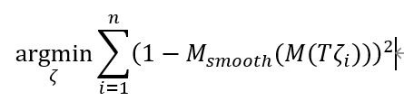![在这里插入图片描述](https://img-blog.csdnimg.cn/7d3794875d894790b52438cd4c244826.png#pic_center)

              static_cast<double>(kPadding),
          (limits.max().y() - world[1]) / limits.resolution() - 0.5 +
              static_cast<double>(kPadding),
          &residual[i]);
      residual[i] = scaling_factor_ * residual[i];
    }
    return true;
  }

我们首先看到的是它把地图做了两次的封装，一次是封装成了一个adapter。注意计算点对应的栅格加了一个很大的数kPadding，然后在adapter会又把这个kPadding减掉，作者不太理解这个操作的意义，如果有读者知道的话还请不吝赐教。第二层封装是为了给地图做插值，就是论文中的它：

这里给不想看源码的同学提供一个介绍的链接（其实是作者自己懒，去百度了一下）：
https://zhuanlan.zhihu.com/p/161177749
这里作者最后提一个问题，希望有大神能给出解释，对于一个栅格地图来说，给定一个点云（n个点），能不能给出误差对于状态的雅可比矩阵的解析形式（用g2o的后遗症），一个n*3的矩阵。作者自己也对这个问题思考了一下发现关键就在于，对于一个已经转换到local坐标系中的点来说，如何给出该栅格地图计算它对应的的误差的解析形式，即下面这个这个函数的中M的解析形式，其中Msmooth代表插值方式，M代表该栅格地图。还请大神不吝赐教。