TF2-Wide&Deep-API

稀疏特征和密集特征:

稀疏特征:
* 离散值特征
* One-hot
* 叉乘
~ 稀疏特征做叉乘获取共现信息
~ 实现记忆效果

稀疏特征的优缺点:
* 优点
~ 对重复样板高校,广泛应用与工业界
* 缺点
~ 需要人工设计
~ 可能会过拟合

密集特征:
* 向量表达
~ 如 [0.1,0.2,0.6]
*word2vec

密集特征的优缺点
* 优点
~ 带有语义信息,不同向量之间有相关性
~ 兼容没有出现过的特征组合
~ 更少的人工参与
* 缺点
~ 过度泛化,推荐不怎么相关的产品

import matplotlib as mpl
import matplotlib.pyplot as plt
%matplotlib inline
import numpy as np
import sklearn
import pandas as pd
import os
import sys
import tensorflow as tf
from tensorflow import keras

#Get Data
from sklearn.datasets import fetch_california_housing
housing = fetch_california_housing()
data = housing.data
target = housing.target
print("data.shape = ",housing.data.shape)
print("target.shape = ",housing.target.shape)


#split train_test data
from sklearn.model_selection import train_test_split

x_train_all , x_test ,y_train_all , y_test = train_test_split(
    data,target,random_state=7,test_size=0.25
)
print("x_train_all.shape = ",x_train_all.shape)
x_train , x_valid , y_train,y_valid = train_test_split(
    x_train_all,y_train_all,random_state = 11,test_size=0.25
)
print("x_train.shape = ",x_train.shape)

data.shape =  (20640, 8)
target.shape =  (20640,)
x_train_all.shape =  (15480, 8)
x_train.shape =  (11610, 8)

#Normarlization
from sklearn.preprocessing import StandardScaler
scalar = StandardScaler()
x_train_scaled = scalar.fit_transform(x_train)
x_valid_scaled = scalar.transform(x_valid)
x_test_scaled = scalar.transform(x_test)

# Built Model

# 函数式api (这里由于是使用wide&deep模型,所以不能使用Sequntial())
input_data = keras.layers.Input(shape=x_train_scaled.shape[1:])
hidden1 = keras.layers.Dense(30,activation="relu")(input_data)
hidden2 = keras.layers.Dense(30,activation="relu")(hidden1)
#复合函数: f(x) = h(g(x))
concat = keras.layers.concatenate([input_data,hidden2])
output = keras.layers.Dense(1)(concat)

#固化Model
model = keras.models.Model(
    inputs = [input_data],
    outputs = [output]
)
#查看模型
model.summary()

#编译模型
model.compile(loss="mean_squared_error",optimizer="sgd")

Model: "model"
__________________________________________________________________________________________________
Layer (type)                    Output Shape         Param #     Connected to                     
==================================================================================================
input_1 (InputLayer)            [(None, 8)]          0                                            
__________________________________________________________________________________________________
dense (Dense)                   (None, 30)           270         input_1[0][0]                    
__________________________________________________________________________________________________
dense_1 (Dense)                 (None, 30)           930         dense[0][0]                      
__________________________________________________________________________________________________
concatenate (Concatenate)       (None, 38)           0           input_1[0][0]                    
                                                                 dense_1[0][0]                    
__________________________________________________________________________________________________
dense_2 (Dense)                 (None, 1)            39          concatenate[0][0]                
==================================================================================================
Total params: 1,239
Trainable params: 1,239
Non-trainable params: 0
__________________________________________________________________________________________________

history = model.fit(
    x_train_scaled,
    y_train,
    validation_data=(x_valid_scaled,y_valid),
    epochs=10,
)

Train on 11610 samples, validate on 3870 samples
Epoch 1/10
11610/11610 [==============================] - 1s 91us/sample - loss: 1.5455 - val_loss: 0.7846
Epoch 2/10
11610/11610 [==============================] - 1s 69us/sample - loss: 0.6806 - val_loss: 0.7090
Epoch 3/10
11610/11610 [==============================] - 1s 72us/sample - loss: 0.6330 - val_loss: 0.6690
Epoch 4/10
11610/11610 [==============================] - 1s 69us/sample - loss: 0.5998 - val_loss: 0.6382
Epoch 5/10
11610/11610 [==============================] - 1s 72us/sample - loss: 0.5751 - val_loss: 0.6145
Epoch 6/10
11610/11610 [==============================] - 1s 71us/sample - loss: 0.5550 - val_loss: 0.5942
Epoch 7/10
11610/11610 [==============================] - 1s 69us/sample - loss: 0.5383 - val_loss: 0.5745
Epoch 8/10
11610/11610 [==============================] - 1s 69us/sample - loss: 0.5245 - val_loss: 0.5609
Epoch 9/10
11610/11610 [==============================] - 1s 71us/sample - loss: 0.5124 - val_loss: 0.5480
Epoch 10/10
11610/11610 [==============================] - 1s 68us/sample - loss: 0.5019 - val_loss: 0.5395

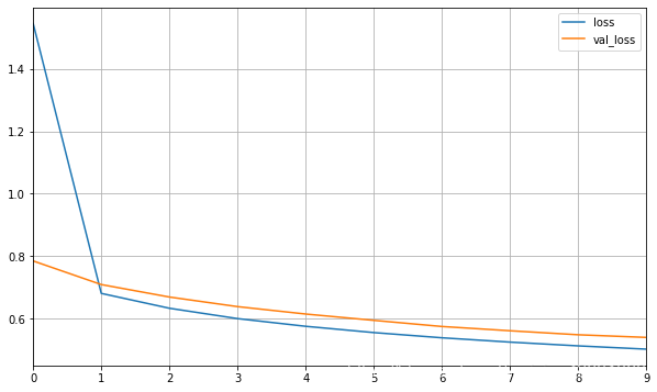
def plot_learning_curves(history):
    pd.DataFrame(history.history).plot(figsize=(10,6))
    plt.grid(True)
#     plt.gca().set_ylim(0,1)
    plt.show()
plot_learning_curves(history)

model.evaluate(x_test_scaled,y_test)

5160/5160 [==============================] - 0s 33us/sample - loss: 0.5178





0.5177843339683473