运用scikit-learn库进行线性和非线性分类

鸢尾花数据是进行机器学习常用的数据之一，本文就鸢尾花数据对分类进行系统的学习。鸢尾花数据获得来自http://archive.ics.uci.edu/ml/machine-learning-databases/iris/iris.data。
数据分类分为线性分类和非线性分类。线性分类分为感知器算法、Logistic回归、SVM（支持向量机）、决策树、随机森林等；非线性分类有核SVM、K近邻算法。

一、线性分类

（一）感知器算法

在对数据进行分类之前，先对数据进行预处理。

from sklearn import datasets
import numpy as np
# 鸢尾花数据集包含在sklearn中
iris = datasets.load_iris()
# 获取特征矩阵（花瓣长度和花瓣宽度）
X = iris.data[:,[2,3]]
# 获取花朵的类标
y = iris.target

# 将数据集划分为训练数据集和测试数据集
from sklearn.cross_validation import train_test_split
# test_size = 0.3表示选取30%的数据集作为测试数据集， 
#  random_state = 0表示每次选取都重新排列训练数据集
X_train, X_test, y_train, y_test = train_test_split(X, y, test_size = 0.3, random_state = 0)

# 对特征矩阵进行标准化
from sklearn.preprocessing import StandardScaler
sc = StandardScaler()
# 获取每个特征的均值和标准差
sc.fit(X_train)
# 按每个特征的均值和标准差对每个特征进行标准化
X_train_std = sc.transform(X_train)
# 对获得的均值和标准差对测试数据集进行标准化
X_test_std = sc.transform(X_test)

# 设置 决策区域 图函数
from matplotlib.colors import ListedColormap
import matplotlib.pyplot as plt
import warnings


def versiontuple(v):
    return tuple(map(int, (v.split("."))))


def plot_decision_regions(X, y, classifier, test_idx=None, resolution=0.02):

    # setup marker generator and color map
    markers = ('s', 'x', 'o', '^', 'v')
    colors = ('red', 'blue', 'lightgreen', 'gray', 'cyan')
    cmap = ListedColormap(colors[:len(np.unique(y))])

    # plot the decision surface
    x1_min, x1_max = X[:, 0].min() - 1, X[:, 0].max() + 1
    x2_min, x2_max = X[:, 1].min() - 1, X[:, 1].max() + 1
    xx1, xx2 = np.meshgrid(np.arange(x1_min, x1_max, resolution),
                           np.arange(x2_min, x2_max, resolution))
    Z = classifier.predict(np.array([xx1.ravel(), xx2.ravel()]).T)
    Z = Z.reshape(xx1.shape)
    plt.contourf(xx1, xx2, Z, alpha=0.4, cmap=cmap)
    plt.xlim(xx1.min(), xx1.max())
    plt.ylim(xx2.min(), xx2.max())

    for idx, cl in enumerate(np.unique(y)):
        plt.scatter(x=X[y == cl, 0], y=X[y == cl, 1],
                    alpha=0.8, c=cmap(idx),
                    marker=markers[idx], label=cl)

    # highlight test samples
    if test_idx:
        # plot all samples
        if not versiontuple(np.__version__) >= versiontuple('1.9.0'):
            X_test, y_test = X[list(test_idx), :], y[list(test_idx)]
            warnings.warn('Please update to NumPy 1.9.0 or newer')
        else:
            X_test, y_test = X[test_idx, :], y[test_idx]

        plt.scatter(X_test[:, 0],
                    X_test[:, 1],
                    c='y',
                    alpha=1.0,
                    linewidths=1,
                    marker='v',
                    s=55, label='test set')

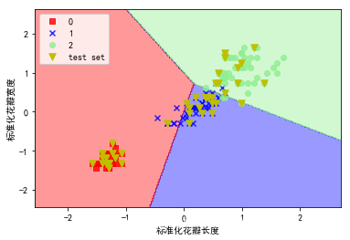
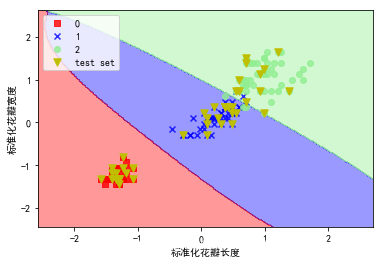
# 使用感知器规则算法对标准化的数据进行训练
from sklearn.linear_model import Perceptron
ppn = Perceptron(n_iter = 40, eta0 = 0.1, random_state = 0)
ppn.fit(X_train_std, y_train)

# 使用测试数据集进行测试
y_pred = ppn.predict(X_test_std)
# 查看错误分类数量
print('错误分类数量：%d' % (y_pred != y_test).sum())

# 查看精确分类率
from sklearn.metrics import accuracy_score
print('精确度: %.2f' % accuracy_score(y_test, y_pred))

# 可视化感知器分类结果
import matplotlib.pyplot as plt
# 使文字可以展示
plt.rcParams['font.sans-serif'] = ['SimHei']
# 使负号可以展示
plt.rcParams['axes.unicode_minus'] = False

# 纵向合并 
X_combined_std = np.vstack((X_train_std, X_test_std))
# 横向合并
y_combined = np.hstack((y_train, y_test))

plot_decision_regions(X = X_combined_std, y = y_combined, classifier = ppn, test_idx = range(105,150))
# 设置x轴标题
plt.xlabel("标准化花瓣长度")
# 设置y轴标题
plt.ylabel('标准化花瓣宽度')
# 设置图例位置
plt.legend(loc = 'upper left')
plt.show()

（二）Logistic回归

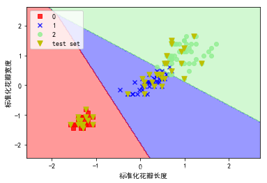
from sklearn.linear_model import LogisticRegression
# C是正则化系数的倒数
lr = LogisticRegression(C = 1000.0, random_state = 0)
lr.fit(X_train_std, y_train)
# 可视化分类结果
plot_decision_regions(X_combined_std, y_combined, classifier = lr, test_idx = range(105, 150))
# 设置x轴标题
plt.xlabel('标准化花瓣长度')
# 设置y轴标题
plt.ylabel('标准化花瓣宽度')
# 设置图例
plt.legend(loc = 'upper left')
plt.show()

（三）SVM（支持向量机）

from sklearn.svm import SVC
svm = SVC(kernel = 'linear', C = 1.0, random_state = 0)
svm.fit(X_train_std, y_train)
# 可视化分类结果
plot_decision_regions(X_combined_std, y_combined, classifier = svm, test_idx = range(105,150))
plt.xlabel('标准化花瓣长度')
plt.ylabel('标准化花瓣宽度')
plt.legend(loc = 'upper left')
plt.show()

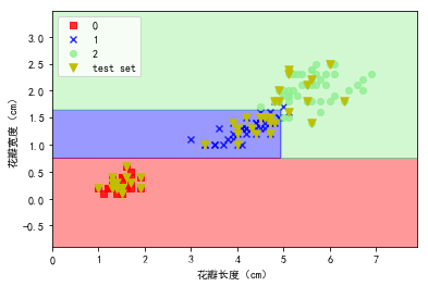
（四）决策树

# 以熵作为不纯度度量标准
from sklearn.tree import DecisionTreeClassifier
tree = DecisionTreeClassifier(criterion = 'entropy', max_depth = 3, random_state = 0)
tree.fit(X_train, y_train)
X_combined = np.vstack((X_train, X_test))
y_combined = np.hstack((y_train, y_test))
# 可视化分类结果
plot_decision_regions(X_combined, y_combined, classifier = tree, test_idx =range(105, 150))
plt.xlabel('花瓣长度（cm）')
plt.ylabel('花瓣宽度（cm）')
plt.legend(loc = 'upper left')
plt.show()

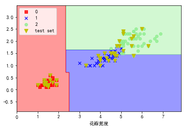
（五）随机森林

from sklearn.ensemble import RandomForestClassifier
#  n_estimator = 10表示有10颗决策树
#  n_jobs = 2表示使用CPU的两个内核
forest = RandomForestClassifier(criterion = 'entropy', n_estimators = 10, random_state = 1, n_jobs = 2)
forest.fit(X_train, y_train)
# 可视化分类结果
plot_decision_regions(X_combined, y_combined, classifier = forest, test_idx = range(105, 150))
plt.xlabel('花瓣长度')
plt.xlabel('花瓣宽度')
plt.legend(loc = 'upper left')
plt.show()

二、非线性分类

（一）核SVM

svm = SVC(kernel = 'rbf', random_state = 0, gamma = 0.2, C = 0.2)
svm.fit(X_train_std, y_train)
# 可视化分类结果
plot_decision_regions(X_combined_std, y_combined,classifier = svm, test_idx = range(105, 150))
plt.xlabel('标准化花瓣长度')
plt.ylabel('标准化花瓣宽度')
plt.legend(loc = 'upper left')
plt.show()

（二）K近邻算法

from sklearn.neighbors import KNeighborsClassifier
knn = KNeighborsClassifier(n_neighbors = 5, p = 2, metric= 'minkowski')
knn.fit(X_train_std, y_train)
# 可视化分类结果
plot_decision_regions(X_combined_std, y_combined, classifier = knn, test_idx= range(105, 150))
plt.xlabel('标准化花瓣长度')
plt.ylabel('标准化花瓣宽度')
plt.legend(loc = 'upper left')
plt.show()