Matlab之有趣实验之画多边形图

目录

实验1-从点云中重建多边形边界

实验2-计算多边形域的近似中间轴

实验3-将2D网格变形为修改后的边界

1.加载数据。 要变形的网格由trife，xfe，yfe定义，它是面-顶点格式的三角剖分。

2.构造背景三角剖分-代表网格边界的点集的约束Delaunay三角剖分。

3.编辑背景三角剖分，以将所需的修改合并到域边界。

4.使用变形的背景三角剖分作为评估基础，将描述符转换回笛卡尔坐标。

---

实验1-从点云中重建多边形边界

此示例突出显示了使用Delaunay三角剖分从点云中重建多边形边界的方法。 重建基于优雅的Crust算法。

% Create a set of points representing the point cloud
numpts = 192;
t = linspace( -pi, pi, numpts+1 )';
t(end) = [];
r = 0.1 + 5*sqrt( cos( 6*t ).^2 + (0.7).^2 );
x = r.*cos(t);
y = r.*sin(t);
ri = randperm(numpts);
x = x(ri);
y = y(ri);

% Construct a Delaunay Triangulation of the point set.
dt = delaunayTriangulation(x,y);
tri = dt(:,:);

% Insert the location of the Voronoi vertices into the existing
% triangulation
V = dt.voronoiDiagram();
% Remove the infinite vertex
V(1,:) = [];
numv = size(V,1);
dt.Points(end+(1:numv),:) = V;

% The Delaunay edges that connect pairs of sample points represent the
% boundary.
delEdges = dt.edges();
validx = delEdges(:,1) <= numpts;
validy = delEdges(:,2) <= numpts;
boundaryEdges = delEdges((validx & validy), :)';
xb = x(boundaryEdges);
yb = y(boundaryEdges);
clf;
triplot(tri,x,y);
axis equal;
hold on;
plot(x,y,'*r');
plot(xb,yb, '-r');
xlabel('Curve reconstruction from a point cloud', 'fontweight','b');
hold off;

效果图如下：

---

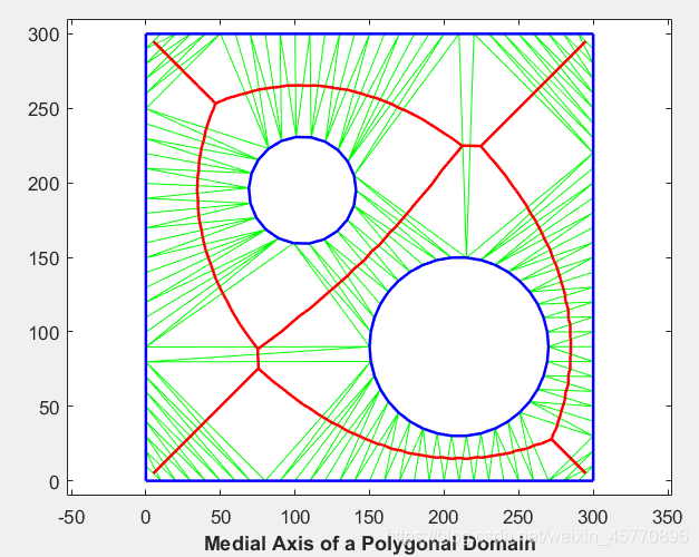
实验2-计算多边形域的近似中间轴

% Construct a constrained Delaunay triangulation of a sample of points
% on the domain boundary.
load trimesh2d
dt = delaunayTriangulation(x,y,Constraints);
inside = dt.isInterior();

% Construct a triangulation to represent the domain triangles.
tr = triangulation(dt(inside, :), dt.Points);

% Construct a set of edges that join the circumcenters of neighboring
% triangles; the additional logic constructs a unique set of such edges.
numt = size(tr,1);
T = (1:numt)';
neigh = tr.neighbors();
cc = tr.circumcenter();
xcc = cc(:,1);
ycc = cc(:,2);
idx1 = T < neigh(:,1);
idx2 = T < neigh(:,2);
idx3 = T < neigh(:,3);
neigh = [T(idx1) neigh(idx1,1); T(idx2) neigh(idx2,2); T(idx3) neigh(idx3,3)]';

% Plot the domain triangles in green, the domain boundary in blue and the
% medial axis in red.
clf;
triplot(tr, 'g');
hold on;
plot(xcc(neigh), ycc(neigh), '-r', 'LineWidth', 1.5);
axis([-10 310 -10 310]);
axis equal;
plot(x(Constraints'),y(Constraints'), '-b', 'LineWidth', 1.5);
xlabel('Medial Axis of a Polygonal Domain', 'fontweight','b');
hold off;

效果图如下：

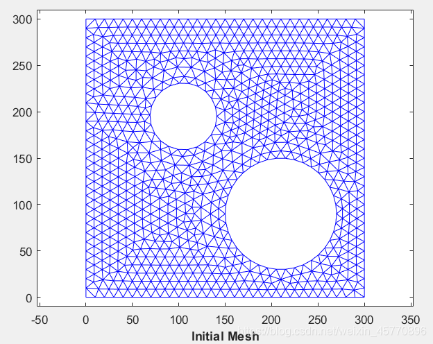
实验3-将2D网格变形为修改后的边界

1.加载数据。 要变形的网格由trife，xfe，yfe定义，它是面-顶点格式的三角剖分。

load trimesh2d
clf;
triplot(trife,xfe,yfe);
axis equal;
axis([-10 310 -10 310]);
axis equal;
xlabel('Initial Mesh', 'fontweight','b');

效果图如下：

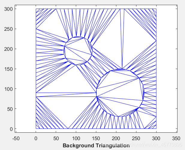
2.构造背景三角剖分-代表网格边界的点集的约束Delaunay三角剖分。

对于网格的每个顶点，计算一个描述符，以定义其相对于背景三角剖分的位置。 描述子是包围的三角形以及相对于该三角形的重心坐标。

dt = delaunayTriangulation(x,y,Constraints);
clf;
triplot(dt);
axis equal;
axis([-10 310 -10 310]);
axis equal;
xlabel('Background Triangulation', 'fontweight','b');
descriptors.tri = pointLocation(dt,xfe, yfe);
descriptors.baryCoords = cartesianToBarycentric(dt,descriptors.tri, [xfe yfe]);

效果图如下：

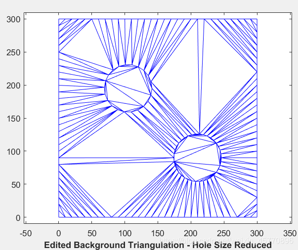
3.编辑背景三角剖分，以将所需的修改合并到域边界。

cc1 = [210 90];
circ1 = (143:180)';
x(circ1) = (x(circ1)-cc1(1))*0.6 + cc1(1);
y(circ1) = (y(circ1)-cc1(2))*0.6 + cc1(2);
tr = triangulation(dt(:,:),x,y);
clf;
triplot(tr);
axis([-10 310 -10 310]);
axis equal;
xlabel('Edited Background Triangulation - Hole Size Reduced', 'fontweight','b');

效果图如下：

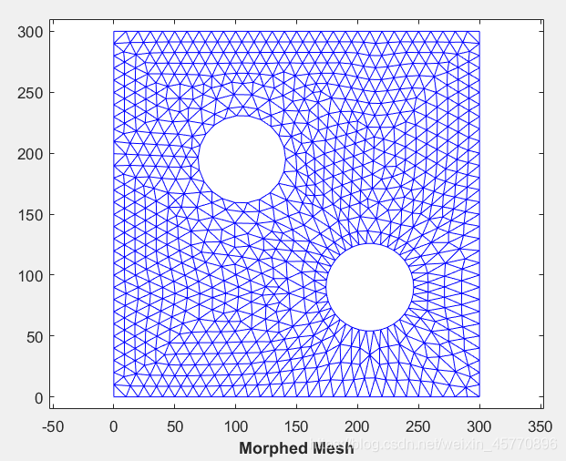
4.使用变形的背景三角剖分作为评估基础，将描述符转换回笛卡尔坐标。

Xnew = barycentricToCartesian(tr,descriptors.tri, descriptors.baryCoords);
tr = triangulation(trife, Xnew);
clf;
triplot(tr);
axis([-10 310 -10 310]);
axis equal;
xlabel('Morphed Mesh', 'fontweight','b');

效果图如下：