


!pip install jupyter_contrib_nbextensions
!pip install -i https://pypi.tuna.tsinghua.edu.cn/simple jupyter_contrib_nbextensions
jupyter contrib nbextension install --user
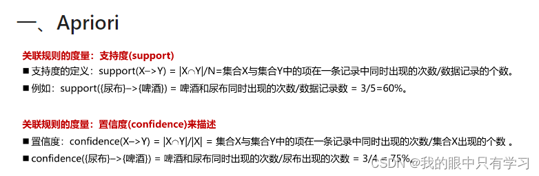
一、Apriori
1.1. 用自写函数
import pandas as pd
import numpy as np

#导入数据集模块
def load_data_set():
    """
    Load a sample data set (From Data Mining: Concepts and Techniques, 3th Edition)
    Returns:
    A data set: A list of transactions. Each transaction contains several items.
    """
    data = pd.read_excel('./Data/orders.xls')
    data_set = np.array(data)
    return data_set

def create_C1(data_set):
    """
    Create frequent candidate 1-itemset C1 by scaning data set.
    Args:
    data_set: A list of transactions. Each transaction contains several items.
    Returns:
    C1: A set which contains all frequent candidate 1-itemsets
    """
    C1 = set()  # 生成空集合
    for t in data_set:
        for item in t:
            item_set = frozenset([item])
            C1.add(item_set)
    return C1

c1 = create_C1(load_data_set())
print(c1)

def is_apriori(Ck_item, Lksub1):
    """
    Judge whether a frequent candidate k-itemset satisfy Apriori property.
    Args:
    Ck_item: a frequent candidate k-itemset in Ck which contains all frequent
    candidate k-itemsets.
    Lksub1: Lk-1, a set which contains all frequent candidate (k-1)-itemsets.
    Returns:
    True: satisfying Apriori property.
    False: Not satisfying Apriori property.
    """
    for item in Ck_item:
        sub_Ck = Ck_item - frozenset([item])
        if sub_Ck not in Lksub1:  #
            return False
        return True

def create_Ck(Lksub1, k):
    """
    Create Ck, a set which contains all all frequent candidate k-itemsets
    by Lk-1's own connection operation.
    Args:
    Lksub1: Lk-1, a set which contains all frequent candidate (k-1)-itemsets.
    Ck
    126
    k: the item number of a frequent itemset.
    Return:
    Ck: a set which contains all all frequent candidate k-itemsets.
    """
    Ck = set()
    len_Lksub1 = len(Lksub1)
    list_Lksub1 = list(Lksub1)
    for i in range(len_Lksub1):
        for j in range(1, len_Lksub1):
            l1 = list(list_Lksub1[i])
            l2 = list(list_Lksub1[j])
            l1.sort()
            l2.sort()
            if l1[0:k-2] == l2[0:k-2]:
                Ck_item = list_Lksub1[i] | list_Lksub1[j]
                # pruning
                if is_apriori(Ck_item, Lksub1):
                    Ck.add(Ck_item)
    return Ck

def generate_Lk_by_Ck(data_set, Ck, min_support, support_data):
    """
    Generate Lk by executing a pruning policy from Ck.
    Args:
    data_set: A list of transactions. Each transaction contains several items.
    Ck: A set which contains all all frequent candidate k-itemsets.
    min_support: The minimum support.
    support_data: A dictionary. The key is frequent itemset and the value is support.
    Returns:
    Lk: A set which contains all all frequent k-itemsets.
    """
    Lk = set()
    item_count = {}
    for t in data_set:
        for item in Ck:
            if item.issubset(t):
                if item not in item_count:
                    item_count[item] = 1
                else:
                    item_count[item] += 1
            t_num = float(len(data_set))
            for item in item_count:
                # 支持度 = item_count[item] / t_num
                if (item_count[item] / t_num) >= min_support:
                    Lk.add(item)
                support_data[item] = item_count[item] / t_num
    return Lk

def generate_L(data_set, k, min_support):
    """
    Generate all frequent itemsets.
    Args:
    data_set: A list of transactions. Each transaction contains several items.
    k: Maximum number of items for all frequent itemsets.
    min_support: The minimum support.
    Returns:
    L: The list of Lk.
    support_data: A dictionary. The key is frequent itemset and the value is support.
    """
    support_data = {}
    C1 = create_C1(data_set)  # 线创建候选1项集
    L1 = generate_Lk_by_Ck(data_set, C1, min_support, support_data) # 通过C1创建频繁1项集
    Lksub1 = L1.copy()
    L = []
    L.append(Lksub1)
    for i in range(2, k+1):        # 循环创建候选集和频繁集
        Ci = create_Ck(Lksub1, i)  # 创建候选集
        Li = generate_Lk_by_Ck(data_set, Ci, min_support, support_data)  # 创建频繁项集
        Lksub1 = Li.copy()  # 低阶频繁集作为下一阶频繁集继续循环
        L.append(Lksub1)
    return L, support_data

def generate_big_rules(L, support_data, min_conf):
    """
    Generate big rules from frequent itemsets.
    Args:
    L: The list of Lk.
    127
    support_data: A dictionary. The key is frequent itemset and the value is support.
    min_conf: Minimal confidence.
    Returns:
    big_rule_list: A list which contains all big rules. Each big rule is represented
    as a 3-tuple.
    """
    big_rule_list = []
    sub_set_list = []
    for i in range(0, len(L)):
        for freq_set in L[i]:
            for sub_set in sub_set_list:
                if sub_set.issubset(freq_set):
                    conf = support_data[freq_set] / support_data[freq_set - sub_set]
                    big_rule = (freq_set - sub_set, sub_set, conf)
                    if conf >= min_conf and big_rule not in big_rule_list:
                        # print freq_set-sub_set, " => ", sub_set, "conf: ", conf
                        big_rule_list.append(big_rule)
            sub_set_list.append(freq_set)
    return big_rule_list
{frozenset({'面包'}), frozenset({'啤酒'}), frozenset({'可乐'}), frozenset({'鸡蛋'}), frozenset({'尿布'}), frozenset({'牛奶'})}
data_set = load_data_set() # 获取数据


# 设置最小支持度0.2,生成频繁项集和支持度数据
L, support_data = generate_L(data_set, k=3, min_support=0.6)
# 设置最小置信度0.7,生成强规则
big_rules_list = generate_big_rules(L, support_data, min_conf=0.7)
for Lk in L:
    print("="*50)
    print("frequent " + str(len(list(Lk))) + "-itemsets\t\tsupport")
    print("="*50)
    for freq_set in Lk:
        print(freq_set, support_data[freq_set])

print("=" * 50)
print("Big Rules")
for item in big_rules_list:
    print(item[0], "=>", item[1], "conf: ", item[2])
==================================================
frequent 4-itemsets		support
==================================================
frozenset({'啤酒'}) 0.75
frozenset({'面包'}) 0.75
frozenset({'尿布'}) 1.0
frozenset({'牛奶'}) 0.75
==================================================
frequent 3-itemsets		support
==================================================
frozenset({'尿布', '面包'}) 0.75
frozenset({'啤酒', '尿布'}) 0.75
frozenset({'牛奶', '尿布'}) 0.75
==================================================
frequent 0-itemsets		support
==================================================
==================================================
Big Rules
frozenset({'尿布'}) => frozenset({'面包'}) conf:  0.75
frozenset({'面包'}) => frozenset({'尿布'}) conf:  1.0
frozenset({'尿布'}) => frozenset({'啤酒'}) conf:  0.75
frozenset({'啤酒'}) => frozenset({'尿布'}) conf:  1.0
frozenset({'牛奶'}) => frozenset({'尿布'}) conf:  1.0
frozenset({'尿布'}) => frozenset({'牛奶'}) conf:  0.75
1.2. 用第三方库
!pip install efficient_apriori
Looking in indexes: https://pypi.tuna.tsinghua.edu.cn/simple
Collecting efficient_apriori
  Downloading https://pypi.tuna.tsinghua.edu.cn/packages/20/5b/a93622c9cc91fc4fb5c29bfeb8689ec4bf1e2b3d0f3579f34975051e6716/efficient_apriori-2.0.1-py3-none-any.whl (14 kB)
Installing collected packages: efficient-apriori
Successfully installed efficient-apriori-2.0.1
apriori(transactions: Iterable[Union[set, tuple, list]], min_support: float = 0.5, min_confidence: float = 0.5, max_length: int = 8, verbosity: int = 0, output_transaction_ids: bool = False)
import efficient_apriori.apriori as aprio
aprio?
import efficient_apriori.apriori as aprio
itemsets, rules = aprio(data_set.tolist(), min_confidence=1)
itemsets
{1: {('牛奶',): 4, ('面包',): 4, ('尿布',): 4, ('啤酒',): 3},
 2: {('啤酒', '尿布'): 3, ('尿布', '牛奶'): 3, ('尿布', '面包'): 3, ('牛奶', '面包'): 3}}
rules
[{啤酒} -> {尿布}]
1.3. FP-Growth
import os
import time
from tqdm import tqdm

def load_data(path):#根据路径加载数据集
# 	ans=[]#将数据保存到该数组
# 	if path.split(".")[-1]=="xls":#若路径为药方.xls
# 		from xlrd import open_workbook
# 		import xlwt
# 		workbook=open_workbook(path)
# 		sheet=workbook.sheet_by_index(0)#读取第一个sheet
# 		for i in range(1,sheet.nrows):#忽视header,从第二行开始读数据,第一列为处方ID,第二列为药品清单
# 			temp=sheet.row_values(i)[1].split(";")[:-1]#取该行数据的第二列并以“;”分割为数组
# 			if len(temp)==0: continue
# 			temp=[j.split(":")[0] for j in temp]#将药品后跟着的药品用量去掉
# 			temp=list(set(temp))#去重,排序
# 			temp.sort()
# 			ans.append(temp)#将处理好的数据添加到数组
	if path.split(".")[-1]=="xls":
		import pandas as pd
		ans = pd.read_excel(path,header=None)
		ans = ans.fillna(0)
		ans = ans.values.tolist()
		for lists in ans:
			for each in range(len(lists)):
	 			if lists[each-1] == 0:
	 			 	lists.pop(each-1)
	 			else:
	 			 	continue

	elif path.split(".")[-1]=="csv":
		import csv
		with open(path,"r") as f:
			reader=csv.reader(f)
			for row in reader:
				row=list(set(row))#去重,排序
				row.sort()
				ans.append(row)#将添加好的数据添加到数组

	return ans#返回处理好的数据集,为二维数组

def save_rule(rule,path):#保存结果到txt文件
	with open(path,"w") as f:
		f.write("index  confidence"+"   rules\n")
		index=1
		for item in rule:
			s=" {:<4d}  {:.3f}        {}=>{}\n".format(index,item[2],str(list(item[0])),str(list(item[1])))
			index+=1
			f.write(s)
		f.close()
	print("result saved,path is:{}".format(path))

class Node:
	def __init__(self, node_name,count,parentNode):
		self.name = node_name
		self.count = count
		self.nodeLink = None#根据nideLink可以找到整棵树中所有nodename一样的节点
		self.parent = parentNode#父亲节点
		self.children = {}#子节点{节点名字:节点地址}

class Fp_growth():
	def update_header(self,node, targetNode):#更新headertable中的node节点形成的链表
		while node.nodeLink != None:
			node = node.nodeLink
		node.nodeLink = targetNode

	def update_fptree(self,items, node, headerTable):#用于更新fptree
		if items[0] in node.children:
			# 判断items的第一个结点是否已作为子结点
			node.children[items[0]].count+=1
		else:
			# 创建新的分支
			node.children[items[0]] = Node(items[0],1,node)
			# 更新相应频繁项集的链表,往后添加
			if headerTable[items[0]][1] == None:
				headerTable[items[0]][1] = node.children[items[0]]
			else:
				self.update_header(headerTable[items[0]][1], node.children[items[0]])
			# 递归
		if len(items) > 1:
			self.update_fptree(items[1:], node.children[items[0]], headerTable)

	def create_fptree(self,data_set, min_support,flag=False):#建树主函数
		'''
		根据data_set创建fp树
		header_table结构为
		{"nodename":[num,node],..} 根据node.nodelink可以找到整个树中的所有nodename
		'''
		item_count = {}#统计各项出现次数
		for t in data_set:#第一次遍历,得到频繁一项集
			for item in t:
				if item not in item_count:
					item_count[item]=1
				else:
					item_count[item]+=1
		headerTable={}
		for k in item_count:#剔除不满足最小支持度的项
			if item_count[k] >= min_support:
				headerTable[k]=item_count[k]

		freqItemSet = set(headerTable.keys())#满足最小支持度的频繁项集
		if len(freqItemSet) == 0:
			return None, None
		for k in headerTable:
			headerTable[k] = [headerTable[k], None] # element: [count, node]
		tree_header = Node('head node',1,None)
		if flag:
			ite=tqdm(data_set)
		else:
			ite=data_set
		for t in ite:#第二次遍历,建树
			localD = {}
			for item in t:
				if item in freqItemSet: # 过滤,只取该样本中满足最小支持度的频繁项
					localD[item] = headerTable[item][0] # element : count
			if len(localD) > 0:
				# 根据全局频数从大到小对单样本排序
				order_item = [v[0] for v in sorted(localD.items(), key=lambda x:x[1], reverse=True)]
				# 用过滤且排序后的样本更新树
				self.update_fptree(order_item, tree_header, headerTable)
		return tree_header, headerTable

	def find_path(self,node, nodepath):
		'''
		获取条件模式基,递归将node的父节点添加到路径
		'''
		if node.parent != None:
			nodepath.append(node.parent.name)
			self.find_path(node.parent, nodepath)

	def find_cond_pattern_base(self,node_name, headerTable):
		'''
		根据节点名字,找出所有条件模式基
		'''
		treeNode = headerTable[node_name][1]
		cond_pat_base = {}#保存所有条件模式基
		while treeNode != None:
			nodepath = []
			self.find_path(treeNode, nodepath)
			if len(nodepath) > 1:
				cond_pat_base[frozenset(nodepath[:-1])] = treeNode.count
			treeNode = treeNode.nodeLink
		return cond_pat_base

	def create_cond_fptree(self,headerTable, min_support, temp, freq_items,support_data):
		# 创建条件模式树,最开始的频繁项集是headerTable中的各元素
		freqs = [v[0] for v in sorted(headerTable.items(), key=lambda p:p[1][0])] # 根据频繁项的总频次排序
		for freq in freqs: # 对每个频繁项
			freq_set = temp.copy()
			freq_set.add(freq)
			freq_items.add(frozenset(freq_set))
			if frozenset(freq_set) not in support_data:#检查该频繁项是否在support_data中
				support_data[frozenset(freq_set)]=headerTable[freq][0]
			else:
				support_data[frozenset(freq_set)]+=headerTable[freq][0]

			cond_pat_base = self.find_cond_pattern_base(freq, headerTable)#寻找到所有条件模式基
			cond_pat_dataset=[]#将条件模式基字典转化为数组
			for item in cond_pat_base:
				item_temp=list(item)
				item_temp.sort()
				for i in range(cond_pat_base[item]):
					cond_pat_dataset.append(item_temp)
			#创建条件模式树
			cond_tree, cur_headtable = self.create_fptree(cond_pat_dataset, min_support)
			if cur_headtable != None:
				self.create_cond_fptree(cur_headtable, min_support, freq_set, freq_items,support_data) # 递归挖掘条件FP树

	def generate_L(self,data_set,min_support):
		freqItemSet=set()
		support_data={}
		tree_header,headerTable=self.create_fptree(data_set,min_support,flag=True)#创建数据集的fptree
		#创建各频繁一项的fptree,并挖掘频繁项并保存支持度计数
		self.create_cond_fptree(headerTable, min_support, set(), freqItemSet,support_data)

		max_l=0
		for i in freqItemSet:#将频繁项根据大小保存到指定的容器L中
			if len(i)>max_l:max_l=len(i)
		L=[set() for _ in range(max_l)]
		for i in freqItemSet:
			L[len(i)-1].add(i)
		for i in range(len(L)):
			print("frequent item {}:{}".format(i+1,len(L[i])))
		return L,support_data

	def generate_R(self,data_set, min_support, min_conf):
		L,support_data=self.generate_L(data_set,min_support)
		rule_list = []
		sub_set_list = []
		for i in range(0, len(L)):
			for freq_set in L[i]:
				for sub_set in sub_set_list:
					if sub_set.issubset(freq_set) and freq_set-sub_set in support_data:#and freq_set-sub_set in support_data
						conf = support_data[freq_set] / support_data[freq_set - sub_set]
						big_rule = (freq_set - sub_set, sub_set, conf)
						if conf >= min_conf and big_rule not in rule_list:
							print(freq_set-sub_set, " => ", sub_set, "conf: ", conf)
							rule_list.append(big_rule)
				sub_set_list.append(freq_set)
		rule_list = sorted(rule_list,key=lambda x:(x[2]),reverse=True)
		return rule_list
os.getcwd()
'D:\\Python\\Jupyter workspace\\学习\\机器学习'
filename="orders.xls"
min_support=0.6#最小支持度
min_conf=1#最小置信度

spend_time=[]
current_path=os.getcwd()
if not os.path.exists(current_path+"/log"):
    os.mkdir("log")

path=current_path+"/Data/"+filename
# print(path)
save_path=current_path+"/log/"+filename.split(".")[0]+"_fpgrowth.txt"

data_set=load_data(path)
# print(data_set)
fp=Fp_growth()
rule_list = fp.generate_R(data_set, min_support, min_conf)
# rule_list
# save_rule(rule_list,save_path)
100%|████████████████████████████████████████████████████████████████████████████████████████████| 5/5 [00:00<?, ?it/s]

frequent item 1:6
frequent item 2:13
frequent item 3:12
frequent item 4:4
frozenset({'鸡蛋'})  =>  frozenset({'啤酒'}) conf:  1.0
frozenset({'鸡蛋'})  =>  frozenset({'尿布'}) conf:  1.0
frozenset({'可乐'})  =>  frozenset({'尿布'}) conf:  1.0
frozenset({'啤酒'})  =>  frozenset({'尿布'}) conf:  1.0
frozenset({'鸡蛋'})  =>  frozenset({'面包'}) conf:  1.0
frozenset({'可乐'})  =>  frozenset({'牛奶'}) conf:  1.0
frozenset({'啤酒', '鸡蛋'})  =>  frozenset({'面包'}) conf:  1.0
frozenset({'鸡蛋', '面包'})  =>  frozenset({'啤酒'}) conf:  1.0
frozenset({'鸡蛋'})  =>  frozenset({'啤酒', '面包'}) conf:  1.0
frozenset({'啤酒', '牛奶'})  =>  frozenset({'尿布'}) conf:  1.0
frozenset({'可乐', '牛奶'})  =>  frozenset({'尿布'}) conf:  1.0
frozenset({'可乐', '尿布'})  =>  frozenset({'牛奶'}) conf:  1.0
frozenset({'可乐'})  =>  frozenset({'牛奶', '尿布'}) conf:  1.0
frozenset({'鸡蛋', '尿布'})  =>  frozenset({'面包'}) conf:  1.0
frozenset({'鸡蛋', '面包'})  =>  frozenset({'尿布'}) conf:  1.0
frozenset({'鸡蛋'})  =>  frozenset({'面包', '尿布'}) conf:  1.0
frozenset({'可乐', '面包'})  =>  frozenset({'牛奶'}) conf:  1.0
frozenset({'可乐', '面包'})  =>  frozenset({'尿布'}) conf:  1.0
frozenset({'鸡蛋', '尿布'})  =>  frozenset({'啤酒'}) conf:  1.0
frozenset({'啤酒', '鸡蛋'})  =>  frozenset({'尿布'}) conf:  1.0
frozenset({'鸡蛋'})  =>  frozenset({'啤酒', '尿布'}) conf:  1.0
frozenset({'可乐', '啤酒'})  =>  frozenset({'牛奶'}) conf:  1.0
frozenset({'啤酒', '面包'})  =>  frozenset({'尿布'}) conf:  1.0
frozenset({'可乐', '啤酒'})  =>  frozenset({'尿布'}) conf:  1.0
frozenset({'可乐', '啤酒', '牛奶'})  =>  frozenset({'尿布'}) conf:  1.0
frozenset({'可乐', '啤酒', '尿布'})  =>  frozenset({'牛奶'}) conf:  1.0
frozenset({'可乐', '啤酒'})  =>  frozenset({'牛奶', '尿布'}) conf:  1.0
frozenset({'可乐', '面包', '牛奶'})  =>  frozenset({'尿布'}) conf:  1.0
frozenset({'可乐', '尿布', '面包'})  =>  frozenset({'牛奶'}) conf:  1.0
frozenset({'可乐', '面包'})  =>  frozenset({'牛奶', '尿布'}) conf:  1.0
frozenset({'啤酒', '鸡蛋', '尿布'})  =>  frozenset({'面包'}) conf:  1.0
frozenset({'面包', '鸡蛋', '尿布'})  =>  frozenset({'啤酒'}) conf:  1.0
frozenset({'啤酒', '鸡蛋', '面包'})  =>  frozenset({'尿布'}) conf:  1.0
frozenset({'啤酒', '鸡蛋'})  =>  frozenset({'面包', '尿布'}) conf:  1.0
frozenset({'鸡蛋', '面包'})  =>  frozenset({'啤酒', '尿布'}) conf:  1.0
frozenset({'鸡蛋', '尿布'})  =>  frozenset({'啤酒', '面包'}) conf:  1.0
frozenset({'鸡蛋'})  =>  frozenset({'尿布', '啤酒', '面包'}) conf:  1.0
frozenset({'啤酒', '牛奶', '面包'})  =>  frozenset({'尿布'}) conf:  1.0
二、协同过滤
2.1. UserCF
CF = Collaborative Filter
import numpy as np
import pandas as pd
from math import sqrt
#%% 字典{user:{item:rating}}
critics = {
    'A': {'老炮儿':3.5,'唐人街探案': 1.0},
    'B': {'老炮儿':2.5,'唐人街探案': 3.5,'星球大战': 3.0, '寻龙诀': 3.5,
                  '神探夏洛克': 2.5, '小门神': 3.0},
    'C': {'老炮儿':3.0,'唐人街探案': 3.5,'星球大战': 1.5, '寻龙诀': 5.0,
                     '神探夏洛克': 3.0, '小门神': 3.5},
    'D': {'老炮儿':2.5,'唐人街探案': 3.5,'寻龙诀': 3.5, '神探夏洛克': 4.0},
    'E': {'老炮儿':3.5,'唐人街探案': 2.0,'星球大战': 4.5, '神探夏洛克': 3.5,
                     '小门神': 2.0},
    'F': {'老炮儿':3.0,'唐人街探案': 4.0,'星球大战': 2.0, '寻龙诀': 3.0,
                     '神探夏洛克': 3.0, '小门神': 2.0},
    'G': {'老炮儿':4.5,'唐人街探案': 1.5,'星球大战': 3.0, '寻龙诀': 5.0,
                      '神探夏洛克': 3.5}
    }

# print(critics['A'])

df = pd.DataFrame(critics)
pcu = df.corr()
pci = df.T.corr()

#df = pd.DataFrame(critics)
#%%
#加载数据
# def ratings_pivot_table():
#     ratings_pivot = pd.pivot_table(ratings_data,index="userId",columns="movieId",values="rating")
#     ratings_pivot = ratings_pivot.fillna(0)
#     return ratings_pivot

# ratings_data = pd.read_csv(".\\movie_data\\ratings2.dat")
# ratings_data.columns=["userId","movieId","rating","time"]
# #print(ratings_data.describe())
# ratings_pivot = ratings_pivot_table()

# ratingdict = ratings_pivot.T.to_dict()
#%% 计算相似性 方法一:欧氏距离
from math import sqrt
def sim_distance(dict_user_item_rating, user1, user2):
    si = {}  # 看过的相同的电影片名的字典
    x = dict_user_item_rating[user1] # 先获取用户1的字典
    y = dict_user_item_rating[user2] # 先获取用户2的字典
    for item in x: # 从每一个用户的评分字典 {'老炮儿': 3.5, '唐人街探案': 1.0} 中获取片名
        if x[item]<=0: continue
        if item in y and y[item]>0: si[item] = 1  # 表示这个电影 user2也看过
    # 如果user2没有看过和user1相同的电影
    if len(si) == 0: return 0  # 不能计算距离
    # 计算欧式距离
    sum_of_squares = sum([pow(x[item] - y[item], 2) for item in x if item in y])
    distance = sqrt(sum_of_squares)
    # 计算基于欧式距离的相似度
    sim = 1 / (1 + distance)
    return sim

import numpy as np
# sim_dict = {}
# for user in critics.keys():
#     if user!="A":
#         sim = sim_distance(critics, 'A', user)
#         #print(f"相似度:A-{user}",round(sim_distance(critics, 'A', user),2))
#         sim_dict[user] = sim
# print("欧氏距离相似度:")
# print(sim_dict)

# 皮尔逊相关度
def sim_pearson(prefs, p1, p2):
    si = {}
    for item in prefs[p1]:
        if item in prefs[p2]: si[item] = 1
    if len(si) == 0: return 0
    n = len(si)    # N
    # 计算开始
    sum1 = sum([prefs[p1][it] for it in si])   # X 的和
    sum2 = sum([prefs[p2][it] for it in si])   # Y 的和
    sum1Sq = sum([pow(prefs[p1][it], 2) for it in si])  # X平方的和
    sum2Sq = sum([pow(prefs[p2][it], 2) for it in si])  # Y平方的和
    pSum = sum([prefs[p1][it] * prefs[p2][it] for it in si])  # XY的和
    num = pSum - (sum1 * sum2 / n)   # 分子 : XY的和 - X的和乘Y的和/N
    den = sqrt((sum1Sq - pow(sum1, 2) / n) * (sum2Sq - pow(sum2, 2) / n))  # 分母
    # 计算结束
    if den == 0: return 0
    r = num / den
    return r

# print("皮尔逊相关系数:")
sim_dict = {}
for user in critics.keys():
    if user!="A":
        sim = sim_pearson(critics, 'A', user)
        #print(f"相似度:A-{user}",round(sim_distance(critics, 'A', user),2))
        sim_dict[user] = sim
# print(sim_dict)


# Gets recommendations for a person by using a weighted average
# of every other user's rankings
def getRecommendations(prefs, person, similarity=sim_distance):
    totals = {}
    simSums = {}
    for other in prefs:
        # don't compare me to myself
        if other == person: continue
        sim = similarity(prefs, person, other)
        # ignore scores of zero or lower
        if sim <= 0: continue
        for item in prefs[other]:  # {'老炮儿':2.5,'唐人街探案': 3.5,'星球大战': 3.0, '寻龙诀': 3.5,'神探夏洛克': 2.5, '小门神': 3.0}
            # only score movies I haven't seen yet
            if item not in prefs[person] or prefs[person][item] == 0:
                # Similarity * Score
                totals.setdefault(item, 0)
                totals[item] += prefs[other][item] * sim
                # Sum of similarities
                simSums.setdefault(item, 0)
                simSums[item] += sim
    # Create the normalized list
    rankings = [(total / simSums[item], item) for item, total in totals.items()] # {movie:total_rating}
    # Return the sorted list
    rankings.sort()
    rankings.reverse()
    return rankings

print("使用欧氏距离计算相似度推荐电影:")
for each in critics:
    print(getRecommendations(critics, each, similarity=sim_distance))

print('++++++++++++++++++++++++++++++++++++++++++++++++++')
print("使用皮尔逊相关系数计算相似度推荐电影:")
for each in critics:
    print(getRecommendations(critics, each, similarity=sim_pearson))
使用欧氏距离计算相似度推荐电影:
[(4.152703901679927, '寻龙诀'), (3.304207244554503, '神探夏洛克'), (3.045124682040546, '星球大战'), (2.5333970389243956, '小门神')]
[]
[]
[(2.755812389354129, '星球大战'), (2.604059105293021, '小门神')]
[(4.012499149875063, '寻龙诀')]
[]
[(2.5835231524824045, '小门神')]
++++++++++++++++++++++++++++++++++++++++++++++++++
使用皮尔逊相关系数计算相似度推荐电影:
[(5.0, '寻龙诀'), (3.75, '星球大战'), (3.5, '神探夏洛克'), (2.0, '小门神')]
[]
[]
[(2.9161893198691655, '小门神'), (2.264442333186428, '星球大战')]
[(5.0, '寻龙诀')]
[]
[(2.601108655629999, '小门神')]
2.2. ItemCF
import numpy as np
import pandas as pd

from math import sqrt
#%%
critics = {
    'A': {'老炮儿':3.5,'唐人街探案': 1.0},
    'B': {'老炮儿':2.5,'唐人街探案': 3.5,'星球大战': 3.0, '寻龙诀': 3.5,
                  '神探夏洛克': 2.5, '小门神': 3.0},
    'C': {'老炮儿':3.0,'唐人街探案': 3.5,'星球大战': 1.5, '寻龙诀': 5.0,
                     '神探夏洛克': 3.0, '小门神': 3.5},
    'D': {'老炮儿':2.5,'唐人街探案': 3.5,'寻龙诀': 3.5, '神探夏洛克': 4.0},
    'E': {'老炮儿':3.5,'唐人街探案': 2.0,'星球大战': 4.5, '神探夏洛克': 3.5,
                     '小门神': 2.0},
    'F': {'老炮儿':3.0,'唐人街探案': 4.0,'星球大战': 2.0, '寻龙诀': 3.0,
                     '神探夏洛克': 3.0, '小门神': 2.0},
    'G': {'老炮儿':4.5,'唐人街探案': 1.5,'星球大战': 3.0, '寻龙诀': 5.0,
                      '神探夏洛克': 3.5}
    }

df = pd.DataFrame(critics)
dfcor = df.T.corr()
#%%
#基于物品的列表
def transformPrefs(prefs):
    itemList ={}
    for person in prefs:
        for item in prefs[person]:
            if item not in itemList:
                itemList[item]={}
                #result.setdefault(item,{})
            itemList[item][person]=prefs[person][item]
    return itemList

#{'老炮儿': {'A': 3.5, 'B': 2.5, 'C': 3.0, 'D': 2.5, 'E': 3.5, 'F': 3.0, 'G': 4.5}
#%%
# 皮尔逊相关度
def sim_pearson(prefs, p1, p2):
    si = {}
    X = prefs[p1]
    Y = prefs[p2]
    for item in X:
        if item in Y: si[item] = 1
    if len(si) == 0: return 0
    n = len(si)
    # 计算开始
    SUM_Xi = sum([ X[i] for i in si ])   # SUM_Xi
    SUM_Yi = sum([ Y[i] for i in si ])
    SUM_XX = sum([ X[i]**2 for i in si ])
    SUM_YY = sum([ Y[i]**2 for i in si ])
    SUM_XY = sum([ X[i]*Y[i] for i in si ])
    num = SUM_XY - (SUM_Xi * SUM_Yi / n)
    den = sqrt((SUM_XX - SUM_Xi**2 / n) * (SUM_YY - SUM_Yi**2 / n))
    # 计算结束
    if den == 0: return 0
    r = num / den
    return r

#%% 欧氏距离相关性
def sim_distance(prefs, p1, p2):
    # Get the list of shared_items
    si = {}
    for item in prefs[p1]:
        if item in prefs[p2]: si[item] = 1
    # if they have no ratings in common, return 0
    if len(si) == 0: return 0
    # Add up the squares of all the differences
    sum_of_squares = sum([pow(prefs[p1][item] - prefs[p2][item], 2)
                          for item in prefs[p1] if item in prefs[p2]])
    return 1 / (1 + sqrt(sum_of_squares))


#%% 找最相似的item
def topMatches(prefs,person,n=5,similarity=sim_distance):
    #python列表推导式
    scores=[(similarity(prefs,person,other),other) for other in prefs if other!=person]
    scores.sort()
    scores.reverse()
    return scores[0:n]

#%%
#构建基于物品相似度数据集
def calculateSimilarItems(prefs,n=10):
    result={}
    itemPrefs=transformPrefs(prefs)
    c = 0
    for item in itemPrefs:  # 电影名称
        c += 1
        if c%10==0: print("%d / %d" % (c,len(itemPrefs)))
        scores=topMatches(itemPrefs,item,n=n,similarity=sim_pearson)
        result[item]=scores
    return result

#%%
#基于物品的推荐
def getRecommendedItems(prefs,itemMatch,user):
    userRatings=prefs[user]
    scores={}
    totalSim={}
# Loop over items rated by this user
    for (item,rating) in userRatings.items( ): #(老炮儿,3.5)
        # Loop over items similar to this one
        for (similarity,item2) in itemMatch[item]:  #  (0.3567891723253309, '神探夏洛克')
            # Ignore if this user has already rated this item
            if item2 in userRatings: continue
            # Weighted sum of rating times similarity
            scores.setdefault(item2,0)
            scores[item2]+=similarity*rating

# Divide each total score by total weighting to get an average
    rankings=[(score,item) for item,score in scores.items()]

# Return the rankings from highest to lowest
    rankings.sort()
    rankings.reverse( )
    return rankings
print(sim_distance(transformPrefs(critics), '老炮儿', '寻龙诀'))
0.2857142857142857
print(sim_distance(critics, 'A', 'B'))
0.2708131845707603
transformPrefs(critics)
{'老炮儿': {'A': 3.5, 'B': 2.5, 'C': 3.0, 'D': 2.5, 'E': 3.5, 'F': 3.0, 'G': 4.5},
 '唐人街探案': {'A': 1.0,
  'B': 3.5,
  'C': 3.5,
  'D': 3.5,
  'E': 2.0,
  'F': 4.0,
  'G': 1.5},
 '星球大战': {'B': 3.0, 'C': 1.5, 'E': 4.5, 'F': 2.0, 'G': 3.0},
 '寻龙诀': {'B': 3.5, 'C': 5.0, 'D': 3.5, 'F': 3.0, 'G': 5.0},
 '神探夏洛克': {'B': 2.5, 'C': 3.0, 'D': 4.0, 'E': 3.5, 'F': 3.0, 'G': 3.5},
 '小门神': {'B': 3.0, 'C': 3.5, 'E': 2.0, 'F': 2.0}}
calculateSimilarItems(critics)
{'老炮儿': [(0.6506000486323551, '寻龙诀'),
  (0.30073740381625697, '星球大战'),
  (0.25332019855244936, '神探夏洛克'),
  (-0.5443310539518174, '小门神'),
  (-0.7691673662934572, '唐人街探案')],
 '唐人街探案': [(0.3207501495497921, '小门神'),
  (-0.38138503569823695, '神探夏洛克'),
  (-0.6712092659994714, '星球大战'),
  (-0.6855106213838525, '寻龙诀'),
  (-0.7691673662934572, '老炮儿')],
 '星球大战': [(0.4412980119034902, '神探夏洛克'),
  (0.30073740381625697, '老炮儿'),
  (-0.08084520834544433, '寻龙诀'),
  (-0.5459486832355505, '小门神'),
  (-0.6712092659994714, '唐人街探案')],
 '寻龙诀': [(0.8910421112136291, '小门神'),
  (0.6506000486323551, '老炮儿'),
  (0.11720180773462399, '神探夏洛克'),
  (-0.08084520834544433, '星球大战'),
  (-0.6855106213838525, '唐人街探案')],
 '神探夏洛克': [(0.4412980119034902, '星球大战'),
  (0.25332019855244936, '老炮儿'),
  (0.11720180773462399, '寻龙诀'),
  (-0.38138503569823695, '唐人街探案'),
  (-0.5443310539518174, '小门神')],
 '小门神': [(0.8910421112136291, '寻龙诀'),
  (0.3207501495497921, '唐人街探案'),
  (-0.5443310539518174, '老炮儿'),
  (-0.5443310539518174, '神探夏洛克'),
  (-0.5459486832355505, '星球大战')]}
print(getRecommendedItems(critics,calculateSimilarItems(critics),'A'))
[(1.5915895488293903, '寻龙诀'), (0.5052356592353358, '神探夏洛克'), (0.3813716473574279, '星球大战'), (-1.5844085392815686, '小门神')]
三、NLP
3.1. 算法流程

TF-Idf
1、假设我们有以下三个文本
• ‘The sun is shining’
• ‘The weather is sweet’
• 'The sun is shining, the weather is sweet, and one and one is two
2、利用CountVectorizer类得到如下字典
{‘and’: 0,‘two’: 7,‘shining’: 3,‘one’: 2,‘sun’: 4,‘weather’: 8,‘the’: 6,‘sweet’: 5,‘is’: 1}
3、将步骤1的文档转换为矩阵
[[0 1 0 1 1 0 1 0 0]
[0 1 0 0 0 1 1 0 1]
[2 3 2 1 1 1 2 1 1]]
4、计算tf-idf值
我们以is为例进行计算,is对应的是矩阵第二列。
tf值,表示term在该文本中出现的次数,这里即is在文本3出现的次数,很容易看出是3.
idf值,sklearn做了小小的改动,公式是 ( 1 + l o g 1 + n d 1 + d f ( d , t ) ) ∗ n d (1+log\frac{1+n_d}{1+df(d,t)})*n_d (1+log1+df(d,t)1+nd)∗nd. 的意思就是文本总数(number of document),df(d,t)表示包含is 的文件数目,很明显,这里也是3.这样,计算的结果为 3 ∗ ( 1 + l o g 1 + 3 1 + 3 ) = 3 3*(1+log\frac{1+3}{1+3})=3 3∗(1+log1+31+3)=3.
需要注意的是,sklearn对结果进行了正则化处理。
t f − i d f ( d 3 ) n o r m = [ 3.39 , 3.0 , 3.39 , 1.29 , 1.29 , 1.29 , 2.0 , 1.69 , 1.29 ] 3.3 9 2 + 3. 0 2 + 3.3 9 2 + 1.2 9 2 + 1.2 9 2 + 1.2 9 2 + 2. 0 2 + 1.6 9 2 + 1.2 9 2 tf-idf(d3)_{norm}=\frac{[3.39,3.0,3.39,1.29,1.29,1.29,2.0,1.69,1.29]}{\sqrt{3.39^{2}+3.0^{2}+3.39^{2}+1.29^{2}+1.29^{2}+1.29^{2}+2.0^{2}+1.69^{2}+1.29^{2}}} tf−idf(d3)norm=3.392+3.02+3.392+1.292+1.292+1.292+2.02+1.692+1.292[3.39,3.0,3.39,1.29,1.29,1.29,2.0,1.69,1.29]
最终得到的结果为
[[ 0. 0.43 0. 0.56 0.56 0. 0.43 0. 0. ]
[ 0. 0.43 0. 0. 0. 0.56 0.43 0. 0.56]
[ 0.5 0.45 0.5 0.19 0.19 0.19 0.3 0.25 0.19]]
每一行的平方和均为1,这是l2正则化处理的结果。
另外可以看出,原先is的词频是 1 1 3,最终tf-idf值是0.43 0.43 0.45 。
3.2. 字符串处理
str0 = 'here I am'
str0.replace('am','is')
'here I is'
str0.find('I')
5
str0.find('am')
7
# 所以寻找单词的起始位置应当
find_substr = 'am'
str0.find(find_substr)-len(find_substr)+1
6
3.2. 基于NLTK库的自然语言处理
!pip install nltk
Requirement already satisfied: nltk in c:\programdata\anaconda3\lib\site-packages (3.4.5)
Requirement already satisfied: six in c:\programdata\anaconda3\lib\site-packages (from nltk) (1.12.0)
!pip install nltkdata
Requirement already satisfied: nltkdata in c:\users\administered\anaconda3\lib\site-packages (0.0.1)
import nltk as nlt

# index1(需要代理):http://www.nltk.org/nltk_data/
# https://gitcode.net/mirrors/nltk/nltk_data/index.xml
nlt.download()
showing info https://raw.githubusercontent.com/nltk/nltk_data/gh-pages/index.xml


Exception in Tkinter callback
Traceback (most recent call last):
  File "C:\Users\administered\Anaconda3\lib\tkinter\__init__.py", line 1705, in __call__
    return self.func(*args)
  File "C:\Users\administered\Anaconda3\lib\site-packages\nltk\downloader.py", line 1656, in _info_save
    callback(entry.get())
  File "C:\Users\administered\Anaconda3\lib\site-packages\nltk\downloader.py", line 1679, in _set_url
    self._ds.url = url
  File "C:\Users\administered\Anaconda3\lib\site-packages\nltk\downloader.py", line 1052, in _set_url
    self._update_index(url)
  File "C:\Users\administered\Anaconda3\lib\site-packages\nltk\downloader.py", line 962, in _update_index
    ElementTree.parse(urlopen(self._url)).getroot()
  File "C:\Users\administered\Anaconda3\lib\xml\etree\ElementTree.py", line 1197, in parse
    tree.parse(source, parser)
  File "C:\Users\administered\Anaconda3\lib\xml\etree\ElementTree.py", line 598, in parse
    self._root = parser._parse_whole(source)
  File "<string>", line None
xml.etree.ElementTree.ParseError: mismatched tag: line 3, column 230
Exception in Tkinter callback
Traceback (most recent call last):
  File "C:\Users\administered\Anaconda3\lib\tkinter\__init__.py", line 1705, in __call__
    return self.func(*args)
  File "C:\Users\administered\Anaconda3\lib\site-packages\nltk\downloader.py", line 1656, in _info_save
    callback(entry.get())
  File "C:\Users\administered\Anaconda3\lib\site-packages\nltk\downloader.py", line 1679, in _set_url
    self._ds.url = url
  File "C:\Users\administered\Anaconda3\lib\site-packages\nltk\downloader.py", line 1052, in _set_url
    self._update_index(url)
  File "C:\Users\administered\Anaconda3\lib\site-packages\nltk\downloader.py", line 962, in _update_index
    ElementTree.parse(urlopen(self._url)).getroot()
  File "C:\Users\administered\Anaconda3\lib\xml\etree\ElementTree.py", line 1197, in parse
    tree.parse(source, parser)
  File "C:\Users\administered\Anaconda3\lib\xml\etree\ElementTree.py", line 598, in parse
    self._root = parser._parse_whole(source)
  File "<string>", line None
xml.etree.ElementTree.ParseError: mismatched tag: line 109, column 2


True
from nltk.corpus import stopwords

stopwords.fileids()
stopwords.raw('english')
"i\nme\nmy\nmyself\nwe\nour\nours\nourselves\nyou\nyou're\nyou've\nyou'll\nyou'd\nyour\nyours\nyourself\nyourselves\nhe\nhim\nhis\nhimself\nshe\nshe's\nher\nhers\nherself\nit\nit's\nits\nitself\nthey\nthem\ntheir\ntheirs\nthemselves\nwhat\nwhich\nwho\nwhom\nthis\nthat\nthat'll\nthese\nthose\nam\nis\nare\nwas\nwere\nbe\nbeen\nbeing\nhave\nhas\nhad\nhaving\ndo\ndoes\ndid\ndoing\na\nan\nthe\nand\nbut\nif\nor\nbecause\nas\nuntil\nwhile\nof\nat\nby\nfor\nwith\nabout\nagainst\nbetween\ninto\nthrough\nduring\nbefore\nafter\nabove\nbelow\nto\nfrom\nup\ndown\nin\nout\non\noff\nover\nunder\nagain\nfurther\nthen\nonce\nhere\nthere\nwhen\nwhere\nwhy\nhow\nall\nany\nboth\neach\nfew\nmore\nmost\nother\nsome\nsuch\nno\nnor\nnot\nonly\nown\nsame\nso\nthan\ntoo\nvery\ns\nt\ncan\nwill\njust\ndon\ndon't\nshould\nshould've\nnow\nd\nll\nm\no\nre\nve\ny\nain\naren\naren't\ncouldn\ncouldn't\ndidn\ndidn't\ndoesn\ndoesn't\nhadn\nhadn't\nhasn\nhasn't\nhaven\nhaven't\nisn\nisn't\nma\nmightn\nmightn't\nmustn\nmustn't\nneedn\nneedn't\nshan\nshan't\nshouldn\nshouldn't\nwasn\nwasn't\nweren\nweren't\nwon\nwon't\nwouldn\nwouldn't\n"
3.3. 基于jieba库的中文语言处理
!pip install jieba
Collecting jieba
  Downloading https://files.pythonhosted.org/packages/c6/cb/18eeb235f833b726522d7ebed54f2278ce28ba9438e3135ab0278d9792a2/jieba-0.42.1.tar.gz (19.2MB)
Building wheels for collected packages: jieba
  Building wheel for jieba (setup.py): started
  Building wheel for jieba (setup.py): finished with status 'done'
  Created wheel for jieba: filename=jieba-0.42.1-cp37-none-any.whl size=19314482 sha256=d88cbc76981e5eb33fe57e965dffcc114df905e2378309528914de60fb66f885
  Stored in directory: C:\Users\administered\AppData\Local\pip\Cache\wheels\af\e4\8e\5fdd61a6b45032936b8f9ae2044ab33e61577950ce8e0dec29
Successfully built jieba
Installing collected packages: jieba
Successfully installed jieba-0.42.1
四、CV
pip install -i https://pypi.tuna.tsinghua.edu.cn/simple opencv-python==3.4.2.17
pip install -i https://pypi.tuna.tsinghua.edu.cn/simple opencv-contrib-python==3.4.2.17
4.1. 图像处理
import math
import cv2
import numpy as np
import matplotlib.pyplot as plt
from PIL import Image, ImageDraw, ImageFont
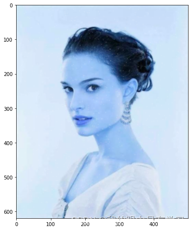
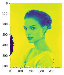
img = cv2.imread('./Data/flower.jpg')
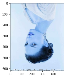
4.1.1. 翻转
img2 = cv2.flip(img,0)  # 0=x轴;1=y轴; -1=xy轴
plt.imshow(img2)
<matplotlib.image.AxesImage at 0x284b0d0d3a0>
Diagonals
796.4923100695951
rows
620
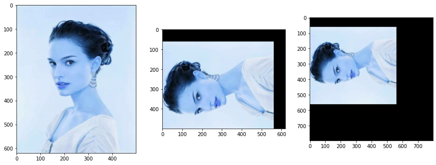
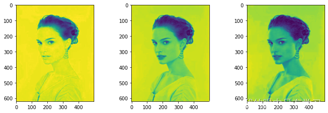
#------------------旋转-------------------------
rows,cols = img.shape[:2]
Diagonals = int(np.sqrt(cols*cols+rows*rows))
# 第一个参数旋转中心,第二个参数旋转角度,第三个参数:缩放比例
M = cv2.getRotationMatrix2D((cols/2,rows/2),90,1)
# 第三个参数:变换后的图像大小
img_swap1 = cv2.warpAffine(img,M,(rows,cols))
# 这里我思考的是将它的对角线进行抽取,旋转的过程中直接将选择角度作用在对角线上,再通过正余弦给它还原回去
img_swap2 = cv2.warpAffine(img,M,(Diagonals,Diagonals))

plt.figure(figsize=(15,12))

plt.subplot(231)
plt.imshow(img)

plt.subplot(232)
plt.imshow(img_swap1)

# 因为留白很丑所以我们给它稍微设计一下
plt.subplot(233)
plt.imshow(img_swap2)
<matplotlib.image.AxesImage at 0x284b4c47670>
4.1.2. 转灰度
cv2.COLOR_RGB2BGRA
2
img3 = cv2.cvtColor(img,cv2.COLOR_RGB2BGRA)
plt.imshow(img3)
<matplotlib.image.AxesImage at 0x21aae225548>
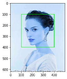
4.1.3. 画方格
cv2.rectangle(img,(100,100),(400,400),(0,255,0),thickness=2)
plt.imshow(img)
<matplotlib.image.AxesImage at 0x24cadb01448>
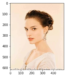
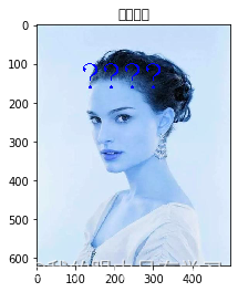
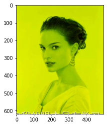
4.1.4. 设置字体
# 图片对象、文本、像素、字体、字体大小、颜色、字体粗细
font = cv2.FONT_HERSHEY_COMPLEX
img = cv2.imread('./Data/flower.jpg')
img = cv2.putText(img, "机器学习", (110, 164), font,3, (0, 0, 255), 2)
plt.title('中文乱码')
plt.imshow(img)
<matplotlib.image.AxesImage at 0x24cadb4a988>


D:\ProgramData\Anaconda3\lib\site-packages\matplotlib\backends\backend_agg.py:211: RuntimeWarning: Glyph 20013 missing from current font.
  font.set_text(s, 0.0, flags=flags)
D:\ProgramData\Anaconda3\lib\site-packages\matplotlib\backends\backend_agg.py:211: RuntimeWarning: Glyph 25991 missing from current font.
  font.set_text(s, 0.0, flags=flags)
D:\ProgramData\Anaconda3\lib\site-packages\matplotlib\backends\backend_agg.py:211: RuntimeWarning: Glyph 20081 missing from current font.
  font.set_text(s, 0.0, flags=flags)
D:\ProgramData\Anaconda3\lib\site-packages\matplotlib\backends\backend_agg.py:211: RuntimeWarning: Glyph 30721 missing from current font.
  font.set_text(s, 0.0, flags=flags)
D:\ProgramData\Anaconda3\lib\site-packages\matplotlib\backends\backend_agg.py:180: RuntimeWarning: Glyph 20013 missing from current font.
  font.set_text(s, 0, flags=flags)
D:\ProgramData\Anaconda3\lib\site-packages\matplotlib\backends\backend_agg.py:180: RuntimeWarning: Glyph 25991 missing from current font.
  font.set_text(s, 0, flags=flags)
D:\ProgramData\Anaconda3\lib\site-packages\matplotlib\backends\backend_agg.py:180: RuntimeWarning: Glyph 20081 missing from current font.
  font.set_text(s, 0, flags=flags)
D:\ProgramData\Anaconda3\lib\site-packages\matplotlib\backends\backend_agg.py:180: RuntimeWarning: Glyph 30721 missing from current font.
  font.set_text(s, 0, flags=flags)
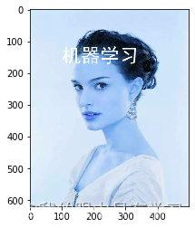
# 自己定义一个add Text的方法
def cv2ImgAddText(img, text, left, top, textColor=(0, 255, 0), textSize=20):
    if (isinstance(img, np.ndarray)):  # 判断是否OpenCV图片类型
        img = Image.fromarray(cv2.cvtColor(img, cv2.COLOR_BGR2RGB))
    # 创建一个可以在给定图像上绘图的对象
    draw = ImageDraw.Draw(img)
    # 字体的格式
    fontStyle = ImageFont.truetype("./simhei.ttf", textSize, encoding="utf-8")
    # 绘制文本
    draw.text((left, top), text, textColor, font=fontStyle)
    # 转换回OpenCV格式
    return cv2.cvtColor(np.asarray(img), cv2.COLOR_RGB2BGR)

img_addtext  = cv2ImgAddText(img, "机器学习", 100, 115, (255, 255 ,255), 60)

titlecn = "图片".encode('gbk').decode(errors='ignore')

plt.imshow(img_addtext)
<matplotlib.image.AxesImage at 0x208e1cecc88>
4.1.5. resize
由于plt是坐标系下画图,所以用plt画图只能观察到坐标系出现了变化,于是我们这里使用cv2.imshow()方法
因为opencv底层是c++写的,所以需要kill掉出来的进程(可以理解为弹窗)
#打印出图片尺寸
img = cv2.imread('./Data/flower.jpg')
print(img.shape)
# # 将图片高和宽分别赋值给x,y
y,x  = img.shape[0:2]
# # 显示原图
cv2.imshow("test",img)
cv2.waitKey()
cv2.destroyAllWindows()
(620, 500, 3)
# # 缩放到原来的二分之一,输出尺寸格式为(宽,高)
img = cv2.resize(img, (int(x / 2), int(y / 2)))
cv2.imshow("test",img)
cv2.waitKey()
cv2.destroyAllWindows()
# # 缩放到原来的二分之一,输出尺寸格式为(宽,高)
img = cv2.resize(img, (int(x * 2), int(y * 2)))
cv2.imshow("test",img)
cv2.waitKey()
cv2.destroyAllWindows()
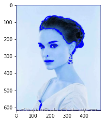
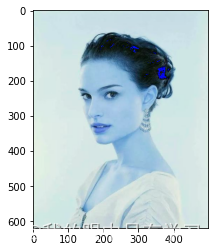
4.1.6. 标记轮廓
img = cv2.imread('./Data/flower.jpg')
gray = cv2.cvtColor(img, cv2.COLOR_BGR2GRAY)
ret, binary = cv2.threshold(gray, 127, 255, cv2.THRESH_BINARY)
contours, hierarchy = cv2.findContours(binary, cv2.RETR_TREE, cv2.CHAIN_APPROX_SIMPLE)
img_contours = cv2.drawContours(img, contours, -1, (0, 0, 255), 3)
plt.imshow(img_contours)
<matplotlib.image.AxesImage at 0x1cd7819cb80>
4.1.7. 平滑噪点
一般情况下,在我们对图形的轮廓识别完成后会通过轮廓对图形进行裁剪,为了使裁剪后的图形边缘不会过于“生硬”,我们就需要对其进行平滑化处理。
除此以外很多图形也存在帧缺失的情况,某一些像素点模糊,黑噪,啥的,为了好看所以我们就需要给他平滑一下。
一般用到的方法就统计学上比较常见的,高斯分布,然后用高斯核像素矩阵平移或者间补来给它“丝滑”一下
img = cv2.imread('./Data/flower.jpg')

y,x  = img.shape[0:2]
for i in range(1000): #生成1000个噪点
    a = np.random.randint(0,y)
    b = np.random.randint(0,x)
    img[a,b] = 255

plt.figure(figsize=(10,8))
plt.imshow(img)
<matplotlib.image.AxesImage at 0x1cd7854b190>

# 可以看到之前密密麻麻的白色噪点多多少少不那么明显了,不过与之对应图形也会变得模糊。。。
blur_img = cv2.blur(img, (3, 3)) #可以更改核的大小
plt.figure(figsize=(10,8))
plt.imshow(blur_img)
<matplotlib.image.AxesImage at 0x1cd76c08100>

# 高斯平滑,也称为高斯滤波
gblur_img = cv2.GaussianBlur(img,(3, 3),100)
plt.figure(figsize=(10,8))
plt.imshow(gblur_img)
<matplotlib.image.AxesImage at 0x1cd782ee7c0>
plt.imshow?
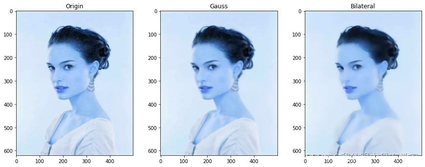
#------------------双边滤波--------------------------
plt.figure(figsize=(15,12))
plt.subplot(2,3,1)
plt.title("Origin",loc='center',y=1)
plt.imshow(img)

img_gauss = cv2.GaussianBlur(img, (5, 5),sigmaX=2,sigmaY=2)
plt.subplot(2,3,2)
plt.title("Gauss",loc='center',y=1)
plt.imshow(img_gauss)

# 这个效果不错欸~
img_bif = cv2.bilateralFilter(src=img_gauss, d=0, sigmaColor=50, sigmaSpace=10)
plt.subplot(2,3,3)
plt.title("Bilateral",loc='center',y=1)
plt.imshow(img_bif)
<matplotlib.image.AxesImage at 0x1cd7e30fcd0>
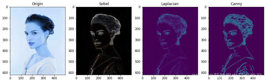
4.1.8. 边缘检测&边缘填充
这它不比什么辣鸡漫水法好十倍?
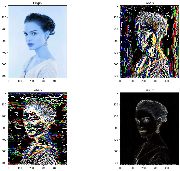
#--------------边缘检测-Sobel---------------
'''
Sobel算子
Sobel算子依然是一种过滤器,只是其是带有方向的。在OpenCV-Python中,
使用Sobel的算子的函数原型如下:
dst = cv2.Sobel(src, ddepth, dx, dy[, dst[, ksize[, scale[, delta[, borderType]]]]])
前四个是必须的参数:
第一个参数是需要处理的图像;
第二个参数是图像的深度,-1表示采用的是与原图像相同的深度。目标图像的深度必须大于等于原图像的深度;
dx和dy表示的是求导的阶数,0表示这个方向上没有求导,一般为0、1、2。
其后是可选的参数:
dst不用解释了;
ksize是Sobel算子的大小,必须为1、3、5、7。
scale是缩放导数的比例常数,默认情况下没有伸缩系数;
delta是一个可选的增量,将会加到最终的dst中,同样,默认情况下没有额外的值加到dst中;
borderType是判断图像边界的模式。这个参数默认值为cv2.BORDER_DEFAULT。
'''
img = cv2.imread('./Data/flower.jpg')
plt.figure(figsize=(15,12))

plt.subplot(2,2,1)
plt.title("Origin",loc='center',y=1)
plt.imshow(img)

sobelx = cv2.Sobel(img, cv2.CV_64F, dx=1, dy=0)  # x方向的
plt.subplot(2,2,2)
plt.title("Sobelx",loc='center',y=1)
plt.imshow(sobelx)

# 使cv2.convertScaleAbs()函数将结果转化为原来的uint8的形式
sobelx = cv2.convertScaleAbs(sobelx)
sobely = cv2.Sobel(img, cv2.CV_64F, dx=0, dy=1)  # y方向的
plt.subplot(2,2,3)
plt.title("Sobely",loc='center',y=1)
plt.imshow(sobely)

sobely = cv2.convertScaleAbs(sobely)
result = cv2.addWeighted(sobelx, 0.5, sobely, 0.5, 0)  # x方向和y方向的梯度权重
plt.subplot(2,2,4)
plt.title("Result",loc='center',y=1)
plt.imshow(result)
Clipping input data to the valid range for imshow with RGB data ([0..1] for floats or [0..255] for integers).
Clipping input data to the valid range for imshow with RGB data ([0..1] for floats or [0..255] for integers).


<matplotlib.image.AxesImage at 0x1cd7cd51220>
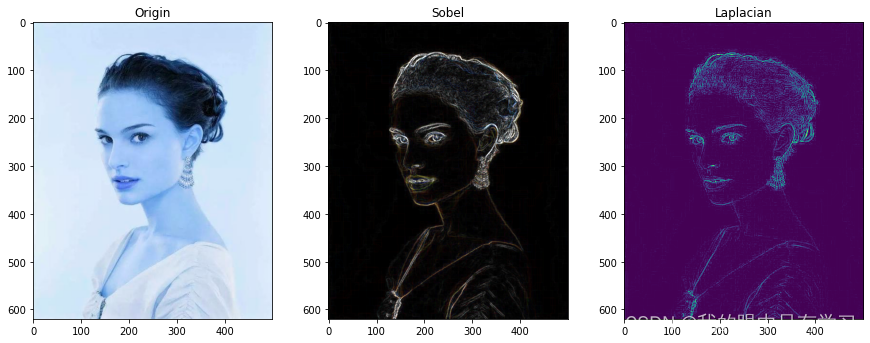
#--------------边缘检测-Laplacian---------------
'''
Laplacian算子
图像中的边缘区域,像素值会发生“跳跃”,对这些像素求导,在其一阶导数在边缘
位置为极值,这就是Sobel算子使用的原理——极值处就是边缘。如果对像素值求二阶导数,
会发现边缘处的导数值为0
Laplace函数实现的方法是先用Sobel 算子计算二阶x和y导数,再求和:
在OpenCV-Python中,Laplace算子的函数原型如下:
dst = cv2.Laplacian(src, ddepth[, dst[, ksize[, scale[, delta[, borderType]]]]])
第一个参数是需要处理的图像;
第二个参数是图像的深度,-1表示采用的是与原图像相同的深度。目标图像的深度必须大于等于原图像的深度;
dst不用解释了;
ksize是算子的大小,必须为1、3、5、7。默认为1。
scale是缩放导数的比例常数,默认情况下没有伸缩系数;
delta是一个可选的增量,将会加到最终的dst中,同样,默认情况下没有额外的值加到dst中;
borderType是判断图像边界的模式。这个参数默认值为cv2.BORDER_DEFAULT。
'''

img = cv2.imread('./Data/flower.jpg')
plt.figure(figsize=(15,12))

plt.subplot(2,3,1)
plt.title("Origin",loc='center',y=1)
plt.imshow(img)

sobelx = cv2.Sobel(img, cv2.CV_64F, dx=1, dy=0)  # x方向的
sobelx = cv2.convertScaleAbs(sobelx)
sobely = cv2.Sobel(img, cv2.CV_64F, dx=0, dy=1)  # y方向的
sobely = cv2.convertScaleAbs(sobely)
result = cv2.addWeighted(sobelx, 0.5, sobely, 0.5, 0)  # x方向和y方向的梯度权重
plt.subplot(2,3,2)
plt.title("Sobel",loc='center',y=1)
plt.imshow(result)

gray = cv2.cvtColor(img, cv2.COLOR_RGB2GRAY)
laplace = cv2.Laplacian(gray, cv2.CV_8U, ksize=3)
plt.subplot(2,3,3)
plt.title("Laplacian",loc='center',y=1)
plt.imshow(laplace)
<matplotlib.image.AxesImage at 0x1cd026c6cd0>
#------------Canny边缘检测-------------------------
'''
Canny边缘检测:
OpenCV-Python中Canny函数的原型为:
edge = cv2.Canny(image, threshold1, threshold2[, edges[, apertureSize[, L2gradient ]]])
必要参数:
第一个参数是需要处理的原图像,该图像必须为单通道的灰度图;
第二个参数是阈值1;
第三个参数是阈值2。
其中较大的阈值2用于检测图像中明显的边缘,但一般情况下检测的效果不会那么完美
,边缘检测出来是断断续续的。所以这时候用较小的第一个阈
值用于将这些间断的边缘连接起来。
可选参数中apertureSize就是Sobel算子的大小。而L2gradient参数是一个布尔值,
如果为真,则使用更精确的L2范数进行计算(即两个方向的倒数的平方和再开放)
,否则使用L1范数(直接将两个方向导数的绝对值相加)。
函数返回一副二值图,其中包含检测出的边缘。
'''

img = cv2.imread('./Data/flower.jpg')
plt.figure(figsize=(15,12))

plt.subplot(2,4,1)
plt.title("Origin",loc='center',y=1)
plt.imshow(img)

sobelx = cv2.Sobel(img, cv2.CV_64F, dx=1, dy=0)  # x方向的
sobelx = cv2.convertScaleAbs(sobelx)
sobely = cv2.Sobel(img, cv2.CV_64F, dx=0, dy=1)  # y方向的
sobely = cv2.convertScaleAbs(sobely)
result = cv2.addWeighted(sobelx, 0.5, sobely, 0.5, 0)  # x方向和y方向的梯度权重
plt.subplot(2,4,2)
plt.title("Sobel",loc='center',y=1)
plt.imshow(result)

gray = cv2.cvtColor(img, cv2.COLOR_RGB2GRAY)
laplace = cv2.Laplacian(gray, cv2.CV_8U, ksize=3)
plt.subplot(2,4,3)
plt.title("Laplacian",loc='center',y=1)
plt.imshow(laplace)


img_gaussBlur = cv2.GaussianBlur(img,(3,3),0) # 降噪可以减少细微的轮廓
canny=cv2.Canny(img_gaussBlur,30,60)
plt.subplot(2,4,4)
plt.title("Canny",loc='center',y=1)
plt.imshow(canny)
<matplotlib.image.AxesImage at 0x1cd06db9f40>
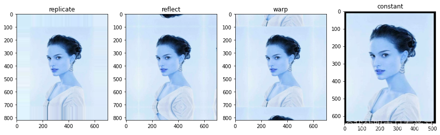
#------------------边界填充-------------------------
#cv2.BORDER_REPLICATE填充,重复最后一个像素,代码及效果:
img_replicate = cv2.copyMakeBorder(img,100,100,100,100,cv2.BORDER_REPLICATE)
#使用cv2.BORDER_REFLECT填充,边界元素的镜像:
img_reflect = cv2.copyMakeBorder(img,100,100,100,100,cv2.BORDER_REFLECT)
#用cv2.BORDER_WRAP填充:
img_warp = cv2.copyMakeBorder(img,100,100,100,100,cv2.BORDER_WRAP)
#用cv2.BORDER_CONSTANT填充,添加一个指定值的边界,默认是黑色:
img_constant = cv2.copyMakeBorder(img,10,10,10,10,cv2.BORDER_CONSTANT)

plt.figure(figsize=(15,12))
plt.subplot(241)
plt.title('replicate')
plt.imshow(img_replicate)

plt.subplot(242)
plt.title('reflect')
plt.imshow(img_reflect)

plt.subplot(243)
plt.title('warp')
plt.imshow(img_warp)

plt.subplot(244)
plt.title('constant')
plt.imshow(img_constant)
<matplotlib.image.AxesImage at 0x284b4590f70>
4.1.9. 锐化
#------------------锐化--------------------------
img = cv2.imread('./Data/flower.jpg')
plt.figure(figsize=(15,15))

plt.subplot(2,2,1)
plt.title("Origin",loc='center',y=1)
plt.imshow(img)

sharpen_op = np.array([[0, 0,1,0, 0], [0, 1,2, 1,0], [1, 2, -16,2,1],[0,1,2,1,0],[0, 0,1,0, 0]], dtype=np.float32)
img_sharpen = cv2.filter2D(img, cv2.CV_32F, sharpen_op)
img_sharpen = cv2.convertScaleAbs(img)
plt.subplot(2,2,2)
plt.title("Sharpen",loc='center',y=1)
plt.imshow(img_sharpen)

# 看结果瞅着没啥区别欸,
<matplotlib.image.AxesImage at 0x284ff1a2280>
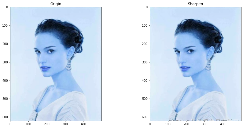
# 咦,好怪再看一眼,还是没啥区别
cv2.imshow('Original',img)
cv2.imshow('Sharpen',img_sharpen)

cv2.waitKey()
cv2.destroyAllWindows()
# 最后一大堆实例,相当于我们自己通过改变图片中的卷积核
# 以此达成在不曲解原图的情况下,实现某种奇妙的【风格迁移】

img = cv2.imread('./Data/flower.jpg')
#自定义卷积核
kernel_sharpen_1 = np.array([
        [-1,-1,-1],
        [-1,9,-1],
        [-1,-1,-1]])
kernel_sharpen_2 = np.array([
        [1,1,1],
        [1,-7,1],
        [1,1,1]])
kernel_sharpen_3 = np.array([
        [-1,-1,-1,-1,-1],
        [-1,2,2,2,-1],
        [-1,2,8,2,-1],
        [-1,2,2,2,-1],
        [-1,-1,-1,-1,-1]])/8.0
#图像锐化
kernel_sharpen_4 = np.array([
        [0,-1,0],
        [-1,5,-1],
        [0,-1,0]])
#图像模糊
kernel_sharpen_5 = np.array([
        [0.0625,0.125,0.0625],
        [0.125,0.25,0.125],
        [0.0625,0.125,0.125]])
#索贝尔
kernel_sharpen_6 = np.array([
        [-1,-2,-1],
        [0,0,0],
        [1,2,1]])
#浮雕
kernel_sharpen_7 = np.array([
        [-2,-1,0],
        [-1,1,1],
        [0,1,2]])
#大纲outline
kernel_sharpen_8 = np.array([
        [-1,-1,-1],
        [-1,8,-1],
        [-1,-1,-1]])
#拉普拉斯算子
kernel_sharpen_9 = np.array([
        [0,1,0],
        [1,-4,1],
        [0,1,0]])
#卷积
output_1 = cv2.filter2D(img,-1,kernel_sharpen_1)
output_2 = cv2.filter2D(img,-1,kernel_sharpen_2)
output_3 = cv2.filter2D(img,-1,kernel_sharpen_3)
output_4 = cv2.filter2D(img,-1,kernel_sharpen_4)
output_5 = cv2.filter2D(img,-1,kernel_sharpen_5)
output_6 = cv2.filter2D(img,-1,kernel_sharpen_6)
output_7 = cv2.filter2D(img,-1,kernel_sharpen_7)
output_8 = cv2.filter2D(img,-1,kernel_sharpen_8)
output_9 = cv2.filter2D(img,-1,kernel_sharpen_9)
#显示锐化效果
cv2.imshow('Original Image',img)
cv2.imshow('sharpen_1 Image',output_1)
cv2.imshow('sharpen_2 Image',output_2)
cv2.imshow('sharpen_3 Image',output_3)
cv2.imshow('sharpen_4 Image',output_4)
cv2.imshow('sharpen_5 Image',output_5)
cv2.imshow('sharpen_6 Image',output_6)
cv2.imshow('sharpen_7 Image',output_7)
cv2.imshow('sharpen_8 Image',output_8)
cv2.imshow('sharpen_9 Image',output_9)

cv2.waitKey()
cv2.destroyAllWindows()
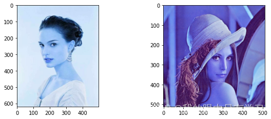
4.1.10. 图像合并
#------------------合并-------------------------
img1 = cv2.imread('./Data/flower.jpg')
img2 = cv2.imread('./Data/lena.jpg')
# (高,宽)
print("图像一的大小{0},图像二的大小{1}".format(img1.shape,img2.shape))
plt.figure(figsize=(10,8))
plt.subplot(221)
plt.imshow(img1)
plt.subplot(222)
plt.imshow(img2)
图像一的大小(620, 500, 3),图像二的大小(512, 512, 3)


<matplotlib.image.AxesImage at 0x284c765cbb0>
#====使用numpy的数组矩阵合并,合并前,纵向合并宽度必须一致,横向合并高度必须一致======
#------------------合并-------------------------
img1 = cv2.imread('./Data/flower.jpg')
img2 = cv2.imread('./Data/lena.jpg')
print("图像一的大小{0},图像二的大小{1}".format(img1.shape,img2.shape))
# resize传入的参数是(宽,高),这里把我一顿好耍
img2 = cv2.resize(img2,(500,512))
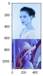
img = np.vstack((img1, img2))# 纵向连接
plt.imshow(img)
<matplotlib.image.AxesImage at 0x284b50f41c0>
#------------------合并-------------------------
img1 = cv2.imread('./Data/flower.jpg')
img2 = cv2.imread('./Data/lena.jpg')
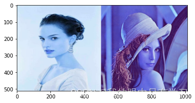
print("图像一的大小{0},图像二的大小{1}".format(img1.shape,img2.shape))
img1 = cv2.resize(img1,(min(img1.shape[1],img2.shape[1]),min(img1.shape[0],img2.shape[0])))
img = np.hstack((img1, img2))#横向连接
plt.imshow(img)
图像一的大小(620, 500, 3),图像二的大小(512, 512, 3)


<matplotlib.image.AxesImage at 0x284b4faa280>
#------------------合并-------------------------
img1 = cv2.imread('./Data/flower.jpg')
img2 = cv2.imread('./Data/lena.jpg')
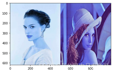
print("图像一的大小{0},图像二的大小{1}".format(img1.shape,img2.shape))
img2 = cv2.resize(img2,(min(img1.shape[1],img2.shape[1]),max(img1.shape[0],img2.shape[0])))
# img = np.concatenate((img1, img2))
img = np.concatenate([img1, img2], axis=1)# 横向连接
plt.imshow(img)
图像一的大小(620, 500, 3),图像二的大小(512, 512, 3)


<matplotlib.image.AxesImage at 0x284b47859d0>
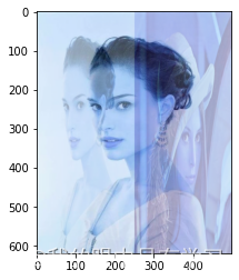
#-------------------加权混合-------------------------
'''
参数1:src1,第一个原数组.
参数2:alpha,第一个数组元素权重
参数3:src2第二个原数组
参数4:beta,第二个数组元素权重
参数5:gamma,图1与图2作和后添加的数值。不要太大,不然图片一片白。总和等于255以上就是纯白色了。
'''
img1 = cv2.imread('./Data/flower.jpg')
img2 = cv2.imread('./Data/lena.jpg')
h, w, _ = img1.shape
# 函数要求两张图必须是同一个size
img2 = cv2.resize(img, (w,h), interpolation=cv2.INTER_AREA)
#print img1.shape, img2.shape
#alpha,beta,gamma可调
alpha = 0.7
beta = 1-alpha
gamma = 0
img = cv2.addWeighted(img1, alpha, img2, beta, gamma)

plt.imshow(img)
<matplotlib.image.AxesImage at 0x284c5fd26d0>
4.1.11. 色彩操作
cv2.cvtColor: The function converts an input image from one color space to another. In case of a transformation
.to-from RGB color space, the order of the channels should be specified explicitly (RGB or BGR).
#------------------------变白,变暗-----------------------------
img = cv2.imread('./Data/flower.jpg')
img = cv2.cvtColor(img,cv2.COLOR_RGB2GRAY)
img = img + 20
plt.imshow(img)
<matplotlib.image.AxesImage at 0x284b51d9370>
#--------------彩色图像R、G、B分量的提取与合并及其相关颜色空间的转化---------

#--------------split—提取R、B、G分量(返回值顺序为:B、G、R)----------
'''
函数原型:split(m, mv=None)
m:彩图矩阵
mv:默认参数
'''
img = cv2.imread('./Data/flower.jpg')
(B,G,R) = cv2.split(img)#提取R、G、B分量

plt.figure(figsize=(12,8))
plt.subplot(231)
plt.imshow(R)
plt.subplot(232)
plt.imshow(G)
plt.subplot(233)
plt.imshow(B)
<matplotlib.image.AxesImage at 0x284b245c190>
#--------------彩色图像R、G、B分量的提取与合并及其相关颜色空间的转化---------

#--------------split—提取R、B、G分量(返回值顺序为:B、G、R)----------
'''
函数原型:split(m, mv=None)
m:彩图矩阵
mv:默认参数
'''
img = cv2.imread('./Data/flower.jpg')
(B,G,R) = cv2.split(img)#提取R、G、B分量
cv2.imshow("Red",R)
cv2.imshow("Green",G)
cv2.imshow("Blue",B)

cv2.waitKey(0)
# cv2.destroyAllWindows()
-1
#--------------merge—合并R、G、B(参数顺序为:B、G、R)-------------
'''
函数原型:merge(mv, dst=None)
m:B、G、R分量
mv:默认参数
'''
# R、G、B分量的提取
(B,G,R) = cv2.split(img) # 提取R、G、B分量
#R、G、B的合并
R = R-20
merged = cv2.merge([B,G,R]) # 合并R、G、B分量
plt.imshow(merged)
<matplotlib.image.AxesImage at 0x284c62a4ac0>
def sigmoid(x):
    s = 1 / (1 + np.exp(-x))
    return s
def R_round(x):
    s = np.round(x)*255
    s = s.astype('uint8')
    return s

(B,G,R) = cv2.split(img)#提取R、G、B分量

#R、G、B的合并
R = sigmoid(R)
R = R_round(R)
merged = cv2.merge([B,G,R])#合并R、G、B分量
plt.imshow(merged)
<ipython-input-101-b72abd0feb4d>:2: RuntimeWarning: overflow encountered in exp
  s = 1 / (1 + np.exp(-x))


<matplotlib.image.AxesImage at 0x284c62b7310>
五、作业
5.1. 作业1
import pandas as pd

data_dict = {'A': {'老炮儿': 3.5, '唐人街探案': 1.0}, 'B': {'老炮儿': 2.5, '唐人街探案': 3.5, '星球大战': 3.0, '寻龙诀': 3.5, '神探夏洛克': 2.5, '小门神': 3.0}, 'C': {'老炮儿': 3.0, '唐人街探案': 3.5, '星球大战': 1.5, '寻龙诀': 5.0, '神探夏洛克': 3.0, '小门神': 3.5}, 'D': {'老炮儿': 2.5, '唐人街探案': 3.5,'寻龙诀': 3.5, '神探夏洛克': 4.0}, 'E': {'老炮儿': 3.5, '唐人街探案': 2.0, '星球大战': 4.5, '神探夏洛克': 3.5, '小门神': 2.0}, 'F': {'老炮儿': 3.0, '唐人街探案': 4.0, '星球大战': 2.0, '寻龙诀': 3.0, '神探夏洛克': 3.0, '小门神': 2.0}, 'G': {'老炮儿': 4.5, '唐人街探案': 1.5, '星球大战': 3.0, '寻龙诀': 5.0, '神探夏洛克': 3.5}}
data_dict
{'A': {'老炮儿': 3.5, '唐人街探案': 1.0},
 'B': {'老炮儿': 2.5,
  '唐人街探案': 3.5,
  '星球大战': 3.0,
  '寻龙诀': 3.5,
  '神探夏洛克': 2.5,
  '小门神': 3.0},
 'C': {'老炮儿': 3.0,
  '唐人街探案': 3.5,
  '星球大战': 1.5,
  '寻龙诀': 5.0,
  '神探夏洛克': 3.0,
  '小门神': 3.5},
 'D': {'老炮儿': 2.5, '唐人街探案': 3.5, '寻龙诀': 3.5, '神探夏洛克': 4.0},
 'E': {'老炮儿': 3.5, '唐人街探案': 2.0, '星球大战': 4.5, '神探夏洛克': 3.5, '小门神': 2.0},
 'F': {'老炮儿': 3.0,
  '唐人街探案': 4.0,
  '星球大战': 2.0,
  '寻龙诀': 3.0,
  '神探夏洛克': 3.0,
  '小门神': 2.0},
 'G': {'老炮儿': 4.5, '唐人街探案': 1.5, '星球大战': 3.0, '寻龙诀': 5.0, '神探夏洛克': 3.5}}
from math import sqrt


def similarity_score(person1,person2):

	# Returns ratio Euclidean distance score of person1 and person2

	both_viewed = {}		# To get both rated items by person1 and person2

	for item in dataset[person1]:
		if item in dataset[person2]:
			both_viewed[item] = 1

		# Conditions to check they both have an common rating items
		if len(both_viewed) == 0:
			return 0

		# Finding Euclidean distance
		sum_of_eclidean_distance = []

		for item in dataset[person1]:
			if item in dataset[person2]:
				sum_of_eclidean_distance.append(pow(dataset[person1][item] - dataset[person2][item],2))
		sum_of_eclidean_distance = sum(sum_of_eclidean_distance)
# 		print(1/(1+sqrt(sum_of_eclidean_distance)))
		return 1/(1+sqrt(sum_of_eclidean_distance))


def pearson_correlation(person1,person2):

	# To get both rated items
	both_rated = {}
	for item in dataset[person1]:
		if item in dataset[person2]:
			both_rated[item] = 1

	number_of_ratings = len(both_rated)

	# Checking for number of ratings in common
	if number_of_ratings == 0:
		return 0

	# Add up all the preferences of each user
	person1_preferences_sum = sum([dataset[person1][item] for item in both_rated])
	person2_preferences_sum = sum([dataset[person2][item] for item in both_rated])

	# Sum up the squares of preferences of each user
	person1_square_preferences_sum = sum([pow(dataset[person1][item],2) for item in both_rated])
	person2_square_preferences_sum = sum([pow(dataset[person2][item],2) for item in both_rated])

	# Sum up the product value of both preferences for each item
	product_sum_of_both_users = sum([dataset[person1][item] * dataset[person2][item] for item in both_rated])

	# Calculate the pearson score
	numerator_value = product_sum_of_both_users - (person1_preferences_sum*person2_preferences_sum/number_of_ratings)
	denominator_value = sqrt((person1_square_preferences_sum - pow(person1_preferences_sum,2)/number_of_ratings) * (person2_square_preferences_sum -pow(person2_preferences_sum,2)/number_of_ratings))
	if denominator_value == 0:
		return 0
	else:
		r = numerator_value/denominator_value
		return r

def most_similar_users(person,number_of_users):
	# returns the number_of_users (similar persons) for a given specific person.
	scores = [(pearson_correlation(person,other_person),other_person) for other_person in dataset if  other_person != person ]

	# Sort the similar persons so that highest scores person will appear at the first
	scores.sort()
	scores.reverse()
	return scores[0:number_of_users]

def user_reommendations(person):

	# Gets recommendations for a person by using a weighted average of every other user's rankings
	totals = {}
	simSums = {}
	rankings_list =[]
	for other in dataset:
		# don't compare me to myself
		if other == person:
			continue
		sim = pearson_correlation(person,other)
		#print ">>>>>>>",sim

		# ignore scores of zero or lower
		if sim <=0:
			continue
		for item in dataset[other]:

			# only score movies i haven't seen yet
			if item not in dataset[person] or dataset[person][item] == 0:

			# Similrity * score
				totals.setdefault(item,0)
				totals[item] += dataset[other][item]* sim
				# sum of similarities
				simSums.setdefault(item,0)
				simSums[item]+= sim

		# Create the normalized list

	rankings = [(total/simSums[item],item) for item,total in totals.items()]
	rankings.sort()
	rankings.reverse()
	# returns the recommended items
	recommendataions_list = [recommend_item for score,recommend_item in rankings]
	return rankings


dataset = data_dict
# print(dataset)

for each in dataset:
    print(each+'的相似用户得分为:'+str(most_similar_users(each,1)))
    print(each+'的推荐电影得分为:'+str(user_reommendations(each)))
    print('+++++++++++++++++++++++++++++++++++++++++++++++++++++++++')
A的相似用户得分为:[(1.0, 'G')]
A的推荐电影得分为:[(5.0, '寻龙诀'), (3.75, '星球大战'), (3.5, '神探夏洛克'), (2.0, '小门神')]
+++++++++++++++++++++++++++++++++++++++++++++++++++++++++
B的相似用户得分为:[(0.4950737714883372, 'C')]
B的推荐电影得分为:[]
+++++++++++++++++++++++++++++++++++++++++++++++++++++++++
C的相似用户得分为:[(0.4950737714883372, 'B')]
C的推荐电影得分为:[]
+++++++++++++++++++++++++++++++++++++++++++++++++++++++++
D的相似用户得分为:[(0.22941573387056174, 'B')]
D的推荐电影得分为:[(2.9161893198691655, '小门神'), (2.264442333186428, '星球大战')]
+++++++++++++++++++++++++++++++++++++++++++++++++++++++++
E的相似用户得分为:[(1.0, 'A')]
E的推荐电影得分为:[(5.0, '寻龙诀')]
+++++++++++++++++++++++++++++++++++++++++++++++++++++++++
F的相似用户得分为:[(0.41176470588235276, 'C')]
F的推荐电影得分为:[]
+++++++++++++++++++++++++++++++++++++++++++++++++++++++++
G的相似用户得分为:[(1.0, 'A')]
G的推荐电影得分为:[(2.601108655629999, '小门神')]
+++++++++++++++++++++++++++++++++++++++++++++++++++++++++
5.2. 期中考试
请根据提供的数据,采用机器学习算法建立模型完成下面的任务:
- 通过用户评分数据,建立推荐模型,完成对与你学号相同的用户ID的旅游产品推荐。
- 根据用户评论文本内容,建立分类模型,实现根据文本内容识别旅游产品分类的功能。
注意:
程序代码中的变量需包含你的姓名拼音首字母作为后缀,如“df_tgy”,“X_train_tgy”等。
import pandas as pd

data = pd.read_excel(r'./Data/data.xlsx',header=0)
data.head()
| 用户ID | 产品分类 | 产品名称 | 产品评分 | 产品评论 | |
|---|---|---|---|---|---|
| 0 | 2019443500 | 酒店 | 化州铭丰假日酒店 | 5 | 位置比较好的,就是床硬了点 |
| 1 | 2019443500 | 景区 | 西江温泉度假村 | 5 | 西江温泉度假村是集温泉理疗、旅业饮食、娱乐健身、旅游购物于一体的综合性旅游度假区。西江温泉自... |
| 2 | 2019443500 | 餐饮 | 甜在心扉千层蛋糕(茂名店) | 5 | 榴莲少了点。味道一般喔价格适中 |
| 3 | 2019443500 | 酒店 | 茂名荔晶大酒店 | 4 | 地理位置不错,停车方便 |
| 4 | 2019443500 | 酒店 | 麗枫酒店(茂名电白万达广场店) | 3 | 停车方便,住的舒服。 |
| 表头 | 含义 |
|---|---|
| 用户ID | 数据包含对旅游产品进行过评价的1000名用户的编号(2019443) |
| 产品分类 | 旅游产品的分类,包含“景点”,“酒店”和“餐饮”三大类 |
| 产品名称 | 被评论产品的名称,即酒店名称、景点名称和餐饮名称 |
| 产品评分 | 用户评分数据(5分制) |
| 产品评论 | 用户评论文本 |
任务一
通过用户评分数据,建立推荐模型,完成对与你学号相同的用户ID的旅游产品推荐
考虑到推荐过程主要需要的信息为用户产品体验的评分与产品名称,推荐结果中产品分类和产品名称一一对应,所以将【用户ID】、【产品名称】、【产品评分】提取为字典形式,并以此构建协同过滤矩阵,完成产品推荐过程
设计字典格式为:
{用户1:{产品1:得分1,产品2:得分2,…},用户2:{产品1:得分1,产品2:得分2,…},…}
# 取列
data_todict = data[['用户ID','产品名称','产品评分']]

data_todict.head()
| 用户ID | 产品名称 | 产品评分 | |
|---|---|---|---|
| 0 | 2019443500 | 化州铭丰假日酒店 | 5 |
| 1 | 2019443500 | 西江温泉度假村 | 5 |
| 2 | 2019443500 | 甜在心扉千层蛋糕(茂名店) | 5 |
| 3 | 2019443500 | 茂名荔晶大酒店 | 4 |
| 4 | 2019443500 | 麗枫酒店(茂名电白万达广场店) | 3 |
# 生成字典格式
data_dict = {}
for ID_each in data_todict['用户ID'].unique():
    data_dict[ID_each] = data_todict[data_todict['用户ID']==ID_each][['产品名称','产品评分']].set_index('产品名称').to_dict()['产品评分']

data_dict
{2019443500: {'化州铭丰假日酒店': 5,
  '西江温泉度假村': 5,
  '甜在心扉千层蛋糕(茂名店)': 5,
  '茂名荔晶大酒店': 4,
  '麗枫酒店(茂名电白万达广场店)': 3,
  '中国南极长城站': 5,
  '盛香烧鹅(东方市场店)': 4,
  '贤合庄卤味火锅(电白万达店)': 2,
  '相聚时光(光明店)': 4},
 2019443501: {'石根山': 3,
  '维也纳国际酒店(茂名万达广场店)': 3,
  '古郡水城': 5,
  '优悦西餐厅(维斯顿店)': 5,
  '菠斯蒂蛋糕': 5,
  'Hello炸鸡(方兴店)': 4,
  '椒王火锅(高州店)': 4,
  '瀛食精致料理': 4,
  'LINLEE·手打柠檬茶(文创店)': 4},
 2019443502: {'天马山生态旅游区': 4,
  '小乔紫菜卷(小乔店)': 4,
  '御水古温泉旅游度假区': 5,
  '顺德火焰醉鹅坊(站北五路店)': 4,
  '菠斯蒂蛋糕': 4,
  '麦当劳(明湖店)': 5,
  '三两粉(茂名东汇城店)': 3}},
  ···}
# 与我学号相同的用户ID的旅游产品
data_dict[2019443909]
{'精途酒店(茂名高铁火车站店)': 3,
 '维也纳国际酒店(茂名万达广场店)': 3,
 '渔港公园': 4,
 '御水古温泉旅游度假区': 3,
 '相聚时光(光明店)': 5,
 '汉宫传承隆江猪脚饭(上排垌店)': 4,
 '贤合庄卤味火锅(电白万达店)': 3,
 '顺德火焰醉鹅坊(站北五路店)': 3,
 '悦创小鹅鹅桂林米粉(双山一路店)': 5}
import numpy as np
import pandas as pd

from math import sqrt

def sim_distance(dict_user_item_rating, user1, user2):
    si = {}  # 看过的相同的电影片名的字典
    x = dict_user_item_rating[user1] # 先获取用户1的字典
    y = dict_user_item_rating[user2] # 先获取用户2的字典
    for item in x: # 从每一个用户的评分字典 {'老炮儿': 3.5, '唐人街探案': 1.0} 中获取片名
        if x[item]<=0: continue
        if item in y and y[item]>0: si[item] = 1  # 表示这个电影 user2也看过
    # 如果user2没有看过和user1相同的电影
    if len(si) == 0: return 0  # 不能计算距离
    # 计算欧式距离
    sum_of_squares = sum([pow(x[item] - y[item], 2) for item in x if item in y])
    distance = sqrt(sum_of_squares)
    # 计算基于欧式距离的相似度
    sim = 1 / (1 + distance)
    return sim

# 皮尔逊相关度
def sim_pearson(prefs, p1, p2):
    si = {}
    for item in prefs[p1]:
        if item in prefs[p2]: si[item] = 1
    if len(si) == 0: return 0
    n = len(si)    # N
    # 计算开始
    sum1 = sum([prefs[p1][it] for it in si])   # X 的和
    sum2 = sum([prefs[p2][it] for it in si])   # Y 的和
    sum1Sq = sum([pow(prefs[p1][it], 2) for it in si])  # X平方的和
    sum2Sq = sum([pow(prefs[p2][it], 2) for it in si])  # Y平方的和
    pSum = sum([prefs[p1][it] * prefs[p2][it] for it in si])  # XY的和
    num = pSum - (sum1 * sum2 / n)   # 分子 : XY的和 - X的和乘Y的和/N
    den = sqrt((sum1Sq - pow(sum1, 2) / n) * (sum2Sq - pow(sum2, 2) / n))  # 分母
    # 计算结束
    if den == 0: return 0
    r = num / den
    return r

# Gets recommendations for a person by using a weighted average
# of every other user's rankings
def getRecommendations(prefs, person, similarity=sim_distance):
    totals = {}
    simSums = {}
    for other in prefs:
        # don't compare me to myself
        if other == person: continue
        sim = similarity(prefs, person, other)
        # ignore scores of zero or lower
        if sim <= 0: continue
        for item in prefs[other]:
            # only score movies I haven't seen yet
            if item not in prefs[person] or prefs[person][item] == 0:
                # Similarity * Score
                totals.setdefault(item, 0)
                totals[item] += prefs[other][item] * sim
                # Sum of similarities
                simSums.setdefault(item, 0)
                simSums[item] += sim
    # Create the normalized list
    rankings = [(total / simSums[item], item) for item, total in totals.items()] # {movie:total_rating}
    # Return the sorted list
    rankings.sort()
    rankings.reverse()
    return rankings
# 推荐结果前5(使用欧氏距离)
print('++++++++++++++++++++++++推荐结果前5(使用欧氏距离)++++++++++++++++++++++++')
print(getRecommendations(data_dict, 2019443909, similarity=sim_distance)[:5])

# 推荐结果前5(使用皮尔逊距离)
print('++++++++++++++++++++++++推荐结果前5(使用皮尔逊距离)++++++++++++++++++++++++')
print(getRecommendations(data_dict, 2019443909, similarity=sim_pearson)[:5])
++++++++++++++++++++++++推荐结果前5(使用欧氏距离)++++++++++++++++++++++++
[(5.0, '鼎龙湾高尔夫度假村'), (5.0, '麗枫酒店(茂名高铁站店)'), (5.0, '高州市宝光塔'), (5.0, '高州卡尔顿酒店'), (5.0, '茂名泊愉青年公寓')]
++++++++++++++++++++++++推荐结果前5(使用皮尔逊距离)++++++++++++++++++++++++
[(5.0, '高州仙人洞景区'), (5.0, '金沙湾海滨浴场'), (5.0, '轻住悦享酒店(茂名高铁南站店)'), (5.0, '西江温泉度假村'), (5.0, '茂名熹龙国际大酒店')]
# 推荐结果展示(欧式距离)
print("+"*30+"用户2019443909的"+"推荐结果展示(欧式距离)"+"+"*30)
result_distance = getRecommendations(data_dict, 2019443909, similarity=sim_distance)[:5]
count = 0
for each in result_distance:
    count = count+1
    print("第"+str(count)+"名,推荐分类:"+str(data[data['产品名称']==each[1]]['产品分类'].unique())+',推荐产品:'+str(each[1]))
++++++++++++++++++++++++++++++用户2019443909的推荐结果展示(欧式距离)++++++++++++++++++++++++++++++
第1名,推荐分类:['景区'],推荐产品:鼎龙湾高尔夫度假村
第2名,推荐分类:['酒店'],推荐产品:麗枫酒店(茂名高铁站店)
第3名,推荐分类:['景区'],推荐产品:高州市宝光塔
第4名,推荐分类:['酒店'],推荐产品:高州卡尔顿酒店
第5名,推荐分类:['酒店'],推荐产品:茂名泊愉青年公寓
# 推荐产品分类(皮尔逊距离)
print("+"*30+"用户2019443909的"+"推荐产品分类(皮尔逊距离)"+"+"*30)
result_pearson = getRecommendations(data_dict, 2019443909, similarity=sim_pearson)[:5]
count = 0
for each in result_pearson:
    count = count+1
    print("第"+str(count)+"名,推荐分类:"+str(data[data['产品名称']==each[1]]['产品分类'].unique())+',推荐产品:'+str(each[1]))
++++++++++++++++++++++++++++++用户2019443909的推荐产品分类(皮尔逊距离)++++++++++++++++++++++++++++++
第1名,推荐分类:['景区'],推荐产品:高州仙人洞景区
第2名,推荐分类:['景区'],推荐产品:金沙湾海滨浴场
第3名,推荐分类:['酒店'],推荐产品:轻住悦享酒店(茂名高铁南站店)
第4名,推荐分类:['景区'],推荐产品:西江温泉度假村
第5名,推荐分类:['酒店'],推荐产品:茂名熹龙国际大酒店
任务二
根据用户评论文本内容,建立分类模型,实现根据文本内容识别旅游产品分类的功能
data_cut = data[['产品分类','产品评论']]
data_cut.head()
| 产品分类 | 产品评论 | |
|---|---|---|
| 0 | 酒店 | 位置比较好的,就是床硬了点 |
| 1 | 景区 | 西江温泉度假村是集温泉理疗、旅业饮食、娱乐健身、旅游购物于一体的综合性旅游度假区。西江温泉自... |
| 2 | 餐饮 | 榴莲少了点。味道一般喔价格适中 |
| 3 | 酒店 | 地理位置不错,停车方便 |
| 4 | 酒店 | 停车方便,住的舒服。 |
# 将产品名称写入专用词典
data['产品名称'].to_csv('./期中考试/我的词典_2019443909.csv',index=0,header=0)
import pandas as pd
dictor = pd.read_csv(r'./期中考试/我的词典_2019443909.csv',header=None)

dictor.head()
| 0 | |
|---|---|
| 0 | 化州铭丰假日酒店 |
| 1 | 西江温泉度假村 |
| 2 | 甜在心扉千层蛋糕(茂名店) |
| 3 | 茂名荔晶大酒店 |
| 4 | 麗枫酒店(茂名电白万达广场店) |
!pip install jieba
Collecting jieba
  Downloading https://files.pythonhosted.org/packages/c6/cb/18eeb235f833b726522d7ebed54f2278ce28ba9438e3135ab0278d9792a2/jieba-0.42.1.tar.gz (19.2MB)
Building wheels for collected packages: jieba
  Building wheel for jieba (setup.py): started
  Building wheel for jieba (setup.py): finished with status 'done'
  Created wheel for jieba: filename=jieba-0.42.1-cp37-none-any.whl size=19314482 sha256=3fbeea9be8d134df2976e503de9da3bc07de3ec43318b869da6d520f0e5a4605
  Stored in directory: C:\Users\administered\AppData\Local\pip\Cache\wheels\af\e4\8e\5fdd61a6b45032936b8f9ae2044ab33e61577950ce8e0dec29
Successfully built jieba
Installing collected packages: jieba
Successfully installed jieba-0.42.1
import jieba

jieba.load_userdict("./期中考试/我的词典_2019443909.csv")
count = 0

for each in data_cut['产品评论']:
    data_cut['产品评论'][count] = " ".join(jieba.lcut(each))
    count = count+1

data_cut
Building prefix dict from the default dictionary ...
Loading model from cache C:\Users\11745\AppData\Local\Temp\jieba.cache
Loading model cost 0.761 seconds.
Prefix dict has been built successfully.
D:\Python\Anaconda\lib\site-packages\IPython\core\interactiveshell.py:3437: SettingWithCopyWarning:
A value is trying to be set on a copy of a slice from a DataFrame

See the caveats in the documentation: https://pandas.pydata.org/pandas-docs/stable/user_guide/indexing.html#returning-a-view-versus-a-copy
  exec(code_obj, self.user_global_ns, self.user_ns)
| 产品分类 | 产品评论 | |
|---|---|---|
| 0 | 酒店 | 位置 比较 好 的 , 就是 床硬 了 点 |
| 1 | 景区 | 西江温泉度假村 是 集 温泉 理疗 、 旅业 饮食 、 娱乐 健身 、 旅游 购物 于 一体... |
| 2 | 餐饮 | 榴莲 少 了 点 。 味道 一般 喔 价格 适中 |
| 3 | 酒店 | 地理位置 不错 , 停车 方便 |
| 4 | 酒店 | 停车 方便 , 住 的 舒服 。 |
| ... | ... | ... |
| 9275 | 餐饮 | 态度 差 , 菜量 特别 少 , 还 不 干净 , 有 不 干净 的 东西 也 不换 不 处... |
| 9276 | 餐饮 | # 泡 芙 # # 蛋挞 # |
| 9277 | 餐饮 | 个人感觉 整体 体验 感觉 一般般 吧 。 |
| 9278 | 餐饮 | 好 |
| 9279 | 餐饮 | 很 满意 的 一次 就餐 体验 , 整体 评价 的话 我 觉得 : 口味 、 团购 接待 、... |
9280 rows × 2 columns
# 划分测试集和训练集
from sklearn.model_selection import train_test_split
X_train, X_test, y_train, y_test = train_test_split(data_cut['产品评论'], data_cut['产品分类'], test_size=0.2, random_state=2017)
# 查看划分结果
X_train
4946    再次 入住 , 茂名 定点 的 了 , 楼 后面 的 停车场 , 四周 交通 便利 , 购物...
1060                                 环境 优雅 , 就是 空调 不给力 哈哈
87                                                     好吃
7496    # 套餐 : 紫菜 卷   4   选   1 店员 做 得 非常 快 , 效率高 但是 味...
7219    榄 菜 豆角 肉沫饭 之前 吃 过 , 挺好吃 的 , 不过 这次 没有 榄 菜 , 味道 ...
                              ...
8963    茂名 出差 , 看着 也 不远 , 就 直接 过来 了 , 酒店 很 新 , 前台 接待 免...
4274                         好吃 经常 和 家人 来 服务员 小 哥哥 态度 很 好
8584                      满意 , 非常 满意 , 味道 不错 , 小朋友 很 喜欢 吃
7978                    公园 不 大 当时 景色 真的 不错 。 可以 来 这里 逛逛 。
4749              此次 用餐 总体 来说 不错 , 觉得 比较 认可 的 地方 有 : 口味 。
Name: 产品评论, Length: 7424, dtype: object
def readFile(path):
    with open(path, 'r', errors='ignore') as file:  # 文档中编码有些问题,所有用errors过滤错误
        content = file.read()
        return content

# 读取停用词
stwlist=[line.strip() for line in open('stopword.txt','r',encoding='utf-8').readlines()]
# 查看stopwords前五行
stwlist[:5]
['\ufeff,', '?', '、', '。', '“']
# 文本向量化处理
from sklearn.feature_extraction.text import CountVectorizer,TfidfVectorizer

# 词袋
cv=CountVectorizer(min_df=3,
                  max_df=0.5,
                  ngram_range=(1,2),
                  stop_words = stwlist)

train_vec=cv.fit_transform(X_train)
test_vec=cv.transform(X_test)
train_vec.data
array([1, 1, 1, ..., 1, 1, 1], dtype=int64)
#1.导入
from sklearn.naive_bayes import MultinomialNB
#2.创建模型
mNB = MultinomialNB()
#3.训练
mNB.fit(train_vec,y_train)
#4.预测
y_pre_MNB = mNB.predict(test_vec)

#1.导入
from sklearn.neighbors import KNeighborsClassifier
#2.创建模型
knn = KNeighborsClassifier(n_neighbors=5)
#3.训练
knn.fit(train_vec,y_train)
#4.预测
y_pre_knn = knn.predict(test_vec)

#1.导入
from sklearn.linear_model import LogisticRegression
#2.创建模型
Logis = LogisticRegression(random_state=0)
#3.训练
Logis.fit(train_vec,y_train)
#4.预测
y_pre_Log = Logis.predict(test_vec)

#1.导入
from sklearn.tree import DecisionTreeClassifier
#2.创建模型
DT = DecisionTreeClassifier(max_depth=5)
#3.训练
DT.fit(train_vec,y_train)
#4.预测
y_pre_DT = DT.predict(test_vec)

#1.导入
from sklearn.linear_model import SGDClassifier
#2.创建模型
SGD = SGDClassifier(loss="hinge", penalty="l2")
#3.训练
SGD.fit(train_vec,y_train)
#4.预测
y_pre_SGD = SGD.predict(test_vec)

#1.导入
from sklearn.svm import SVC
#2.创建模型
SVC = SVC(C=1,kernel="rbf")
#3.训练
SVC.fit(train_vec,y_train)
#4.预测
y_pre_SVC = SVC.predict(test_vec)

#### 模型检验

import numpy as np
from sklearn.metrics import accuracy_score
from sklearn.metrics import classification_report

import warnings
warnings.filterwarnings("ignore")

print("---------------------------MNB-------------------------------")
print(classification_report(y_test, y_pre_MNB))
print("---------------------------knn-------------------------------")
print(classification_report(y_test, y_pre_knn))
print("---------------------------Logstic---------------------------")
print(classification_report(y_test, y_pre_Log))
print("---------------------------DT--------------------------------")
print(classification_report(y_test, y_pre_DT))
print("---------------------------SGD-------------------------------")
print(classification_report(y_test, y_pre_SGD))
print("---------------------------SVC------------------------------")
print(classification_report(y_test, y_pre_SVC))
---------------------------MNB-------------------------------
              precision    recall  f1-score   support

          景区       0.93      0.77      0.84       230
          酒店       0.87      0.82      0.84       215
          餐饮       0.95      0.99      0.97      1411

    accuracy                           0.94      1856
   macro avg       0.92      0.86      0.89      1856
weighted avg       0.94      0.94      0.94      1856

---------------------------knn-------------------------------
              precision    recall  f1-score   support

          景区       0.74      0.28      0.40       230
          酒店       0.84      0.67      0.75       215
          餐饮       0.86      0.97      0.91      1411

    accuracy                           0.85      1856
   macro avg       0.81      0.64      0.69      1856
weighted avg       0.84      0.85      0.83      1856

---------------------------Logstic---------------------------
              precision    recall  f1-score   support

          景区       0.96      0.69      0.80       230
          酒店       0.92      0.81      0.86       215
          餐饮       0.93      0.99      0.96      1411

    accuracy                           0.93      1856
   macro avg       0.94      0.83      0.88      1856
weighted avg       0.94      0.93      0.93      1856

---------------------------DT--------------------------------
              precision    recall  f1-score   support

          景区       0.96      0.22      0.35       230
          酒店       0.91      0.55      0.69       215
          餐饮       0.84      1.00      0.91      1411

    accuracy                           0.85      1856
   macro avg       0.90      0.59      0.65      1856
weighted avg       0.86      0.85      0.82      1856

---------------------------SGD-------------------------------
              precision    recall  f1-score   support

          景区       0.94      0.71      0.81       230
          酒店       0.90      0.80      0.85       215
          餐饮       0.94      0.99      0.96      1411

    accuracy                           0.93      1856
   macro avg       0.92      0.83      0.87      1856
weighted avg       0.93      0.93      0.93      1856

---------------------------SVC------------------------------
              precision    recall  f1-score   support

          景区       0.98      0.52      0.68       230
          酒店       0.92      0.74      0.82       215
          餐饮       0.90      1.00      0.95      1411

    accuracy                           0.91      1856
   macro avg       0.93      0.75      0.82      1856
weighted avg       0.91      0.91      0.90      1856
# TF-IDF
tdf=TfidfVectorizer(min_df=3,
                  max_df=0.5,
                  ngram_range=(1,2),
                  stop_words = stwlist)

train_vec=tdf.fit_transform(X_train)
test_vec=tdf.transform(X_test)
train_vec.data
array([0.2324165 , 0.35501622, 0.19470487, ..., 0.1971904 , 0.22019233,
       0.13635501])
#1.导入
from sklearn.naive_bayes import MultinomialNB
#2.创建模型
mNB = MultinomialNB()
#3.训练
mNB.fit(train_vec,y_train)
#4.预测
y_pre_MNB = mNB.predict(test_vec)

#1.导入
from sklearn.neighbors import KNeighborsClassifier
#2.创建模型
knn = KNeighborsClassifier(n_neighbors=5)
#3.训练
knn.fit(train_vec,y_train)
#4.预测
y_pre_knn = knn.predict(test_vec)

#1.导入
from sklearn.linear_model import LogisticRegression
#2.创建模型
Logis = LogisticRegression(random_state=0)
#3.训练
Logis.fit(train_vec,y_train)
#4.预测
y_pre_Log = Logis.predict(test_vec)

#1.导入
from sklearn.tree import DecisionTreeClassifier
#2.创建模型
DT = DecisionTreeClassifier(max_depth=5)
#3.训练
DT.fit(train_vec,y_train)
#4.预测
y_pre_DT = DT.predict(test_vec)

#1.导入
from sklearn.linear_model import SGDClassifier
#2.创建模型
SGD = SGDClassifier(loss="hinge", penalty="l2")
#3.训练
SGD.fit(train_vec,y_train)
#4.预测
y_pre_SGD = SGD.predict(test_vec)

#1.导入
from sklearn.svm import SVC
#2.创建模型
SVC = SVC(C=1,kernel="rbf")
#3.训练
SVC.fit(train_vec,y_train)
#4.预测
y_pre_SVC = SVC.predict(test_vec)

#### 6.2.6 模型检验

import numpy as np
from sklearn.metrics import accuracy_score
from sklearn.metrics import classification_report

import warnings
warnings.filterwarnings("ignore")

print("---------------------------MNB-------------------------------")
print(classification_report(y_test, y_pre_MNB))
print("---------------------------knn-------------------------------")
print(classification_report(y_test, y_pre_knn))
print("---------------------------Logstic---------------------------")
print(classification_report(y_test, y_pre_Log))
print("---------------------------DT--------------------------------")
print(classification_report(y_test, y_pre_DT))
print("---------------------------SGD-------------------------------")
print(classification_report(y_test, y_pre_SGD))
print("---------------------------SVC------------------------------")
print(classification_report(y_test, y_pre_SVC))
---------------------------MNB-------------------------------
              precision    recall  f1-score   support

          景区       0.98      0.68      0.81       230
          酒店       0.93      0.79      0.85       215
          餐饮       0.93      1.00      0.96      1411

    accuracy                           0.93      1856
   macro avg       0.95      0.82      0.87      1856
weighted avg       0.94      0.93      0.93      1856

---------------------------knn-------------------------------
              precision    recall  f1-score   support

          景区       0.59      0.12      0.20       230
          酒店       0.74      0.17      0.28       215
          餐饮       0.79      0.99      0.88      1411

    accuracy                           0.78      1856
   macro avg       0.71      0.42      0.45      1856
weighted avg       0.76      0.78      0.72      1856

---------------------------Logstic---------------------------
              precision    recall  f1-score   support

          景区       0.99      0.66      0.79       230
          酒店       0.93      0.79      0.85       215
          餐饮       0.93      1.00      0.96      1411

    accuracy                           0.93      1856
   macro avg       0.95      0.82      0.87      1856
weighted avg       0.93      0.93      0.93      1856

---------------------------DT--------------------------------
              precision    recall  f1-score   support

          景区       0.96      0.20      0.33       230
          酒店       0.91      0.55      0.69       215
          餐饮       0.84      1.00      0.91      1411

    accuracy                           0.85      1856
   macro avg       0.90      0.58      0.64      1856
weighted avg       0.86      0.85      0.81      1856

---------------------------SGD-------------------------------
              precision    recall  f1-score   support

          景区       0.98      0.73      0.83       230
          酒店       0.90      0.82      0.86       215
          餐饮       0.94      0.99      0.96      1411

    accuracy                           0.94      1856
   macro avg       0.94      0.85      0.89      1856
weighted avg       0.94      0.94      0.94      1856

---------------------------SVC------------------------------
              precision    recall  f1-score   support

          景区       0.97      0.68      0.80       230
          酒店       0.91      0.79      0.85       215
          餐饮       0.93      0.99      0.96      1411

    accuracy                           0.93      1856
   macro avg       0.94      0.82      0.87      1856
weighted avg       0.93      0.93      0.93      1856
input_test = "这家的番茄鸡蛋真的超级好吃,唯一的缺点就是川菜太辣了!!!"
input_cut = jieba.lcut(input_test)

#预测 CV-MNG
input_cv = cv.transform(input_cut)
y_pre_MNB = mNB.predict(input_cv)
y_pre_MNB[0]
'餐饮'
#预测 TDF-SGD
input_tdf = tdf.transform(input_cut)
y_pre_SGD = SGD.predict(input_cv)
y_pre_SGD[0]
'餐饮'
# 我们观察到预测结果中SVC的结果,在全部预测【餐饮】的情况下准确率居然高达0.76!
# 于是我们查看一下是否存在样本类别分布不均衡现象

import matplotlib.pyplot as plt
plt.rcParams['font.sans-serif']=['SimHei']     #显示中文
plt.rcParams['axes.unicode_minus']=False       #正常显示负号


data['产品分类'].value_counts().plot(kind='bar')
<matplotlib.axes._subplots.AxesSubplot at 0x1a0ec188>
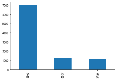
5.3. 作业2
检测 face_detect.jpg
import os
import sys
import cv2
import numpy as np

frame = cv2.imread('./Data/face_detect.jpg')
gray = cv2.cvtColor(frame, cv2.COLOR_BGR2GRAY)
targetdir = './Data/captured/'

face_cascade = cv2.CascadeClassifier(r'.\cascades\haarcascade_frontalface_alt.xml')
faces = face_cascade.detectMultiScale(gray)

count = 1
for (x, y, w, h) in faces:
    cv2.circle(frame, (int(x + w/2), int(y + h/2)), int(max(w,h)/2) , (255, 0, 0), 2)

#     f = cv2.resize(gray[y:y + h, x:x + w], (200, 200))
#     filename = os.path.join(targetdir,"{}.jpg".format(count))
#     cv2.imwrite(filename, f)
#     count += 1
#     print(filename)

cv2.imshow('face', frame)
cv2.waitKey(0)
cv2.destroyAllWindows()
检测 video.mp4
targetdir = './Data/captured/'
face_cascade = cv2.CascadeClassifier(r'.\cascades\haarcascade_frontalface_alt.xml')
camera = cv2.VideoCapture('./Data/video.mp4')

camera.set(3, 1280)
camera.set(4, 720)

cv2.namedWindow('face')
ret, img = camera.read()

count=1
while ret:
    ret, img = camera.read()
    if ret:
        gray = cv2.cvtColor(img, cv2.COLOR_BGR2GRAY)
        faces = face_cascade.detectMultiScale(gray, 1.2, 5, minSize=(50, 50))
        for (x, y, w, h) in faces:
            img = cv2.circle(img, (int(x + w/2), int(y + h/2)), int(max(w,h)/2) , (255, 0, 0), 2)
            roi = gray[y:y + h, x:x + w]

        filename = os.path.join(targetdir,"{}.jpg".format(count))
        cv2.imwrite(filename, img)
        count += 1
        cv2.imshow('face', img)

    pressKey = cv2.waitKey(20)
    if cv2.getWindowProperty('face', cv2.WND_PROP_AUTOSIZE) < 1:
        break
    if pressKey == 27:  # ESC
        print('退出。。。。。')
        break

camera.release()
cv2.destroyAllWindows()
合成检测结果视频
from PIL import Image

im_dir = targetdir
video_dir = './Data/video_return.avi'
fps = 23

im_list = os.listdir(im_dir)
im_list.sort(key=lambda x: int(x.replace("frame","").split('.')[0]))  #看看图片顺序对不
img = Image.open(os.path.join(im_dir,im_list[0]))
img_size = img.size #获得图片分辨率,im_dir文件夹下的图片分辨率需要一致


fourcc = cv2.VideoWriter_fourcc(*'DIVX')
videoWriter = cv2.VideoWriter(video_dir, fourcc, fps, img_size)
count = 1
for i in im_list:
    im_name = os.path.join(im_dir+i)
    frame = cv2.imdecode(np.fromfile(im_name, dtype=np.uint8), -1)
    videoWriter.write(frame)
    count += 1

videoWriter.release()
print('Video return finish!')
因为图 face_detect.jpg 中检测结果不是很理想,于是我们尝试使用CV识别方向的工业级模型yolov5
!git clone https://github.com/ultralytics/yolov5  # clone

!cd yolov5

!pip install -r requirements.txt  # install
!python ./yolov5-face-master/detect_face.py --weights ./yolov5-face-master/weights/yolov5s_face.pt --image ./Data/face_detect.jpg --img-size 640
5.4. 期末考试
建模前的准备
读取数据
import os

PATH = './cats_vs_dogs/'
train_dir = os.path.join(PATH, 'train')
validation_dir = os.path.join(PATH, 'validation')
train_cats_dir = os.path.join(train_dir, 'cats')  # directory with our training cat pictures
train_dogs_dir = os.path.join(train_dir, 'dogs')  # directory with our training dog pictures
validation_cats_dir = os.path.join(validation_dir, 'cats')  # directory with our validation cat pictures
validation_dogs_dir = os.path.join(validation_dir, 'dogs')  # directory with our validation dog pictures
查看数据集分布情况
num_cats_train = len(os.listdir(train_cats_dir))
num_dogs_train = len(os.listdir(train_dogs_dir))

num_cats_val = len(os.listdir(validation_cats_dir))
num_dogs_val = len(os.listdir(validation_dogs_dir))

total_train = num_cats_train + num_dogs_train
total_val = num_cats_val + num_dogs_val

print('total training cat images:', num_cats_train)
print('total training dog images:', num_dogs_train)
print("--")
print('total validation cat images:', num_cats_val)
print('total validation dog images:', num_dogs_val)
print("--")
print("Total training images:", total_train)
print("Total validation images:", total_val)
total training cat images: 990
total training dog images: 990
--
total validation cat images: 500
total validation dog images: 500
--
Total training images: 1980
Total validation images: 1000
我们先通过opencv的SIFT的特征提取实现,来帮我们提取出猫狗在图像上的特征
机器学习方法(使用sklearn)
初步尝试
首先我们尝试一下直接输入数据,并直接进行一维放缩,由此预测结果。
这里我们使用支持向量机(SVM)模型进行预测(此模型多维输入二分类任务表现较好)
import cv2 #opencv库,用于读取图片等操作
import numpy as np
import pandas as pd
from sklearn.preprocessing import StandardScaler #标准差标准化
from sklearn.svm import SVC                      #svm包中SVC用于分类
from sklearn.decomposition import PCA            #特征分解模块的PCA用于降维

def get_data(x,y):
    file_path='./cats_vs_dogs/train/' #设置文件路径(这里为当前目录下的ORL文件夹)
    train_set = pd.DataFrame()     #将train_set转换成DataFrame类型
    target=[]                               #标签列表
    IMG_H = 120
    IMG_W = 100
    for i in ('cat','dog'):            #i用于遍历ORL文件夹中的2个文件夹
        print('Start Get Data From '+ i)
        for j in range(x,y):                #j用于遍历每个文件夹的对应的x到y-1的图片
            target.append(i)                #读入标签(图片文件夹中的人脸是同一个类的)
            img = cv2.imread(file_path+i+'s/'+i+'.'+str(j)+'.jpg',\
            cv2.IMREAD_GRAYSCALE) #读取图片,第二个参数表示以灰度图像读入
            img = cv2.resize(img, (IMG_W,IMG_H)) # 将图片进行放缩(防止矩阵维度过大内存溢出)
            img=img.reshape(1,img.shape[0]*img.shape[1]) #将读入的图片数据转换成一维
            img=pd.DataFrame(img)           #将一维的图片数据转成DataFrame类型
            train_set=pd.concat([train_set,img],axis=0)#按行拼接DataFrame矩阵
#             print('Get Data Finish ' + str(j))
    train_set.index=list(range(0,train_set.shape[0])) #设置 train_set的行索引
    train_set.drop(labels=0,axis=0,inplace=True) #删除行索引为0的行(删除第一行)
    target=pd.DataFrame(target)             #将标签列表转成DataFrame类型
    return train_set,target                 #返回数据集和标签

if __name__ == '__main__':
    #1、获取数据
    data_train,target_train=get_data(0,500) #读取前五张图片为训练集
    data_test,target_test=get_data(501,700)  #读取后五张图片为测试集
    #2、数据标准化 标准差标准化
    stdScaler = StandardScaler().fit(data_train)
    trainStd = stdScaler.transform(data_train)
    #stdScaler = StandardScaler().fit(data_test)
    testStd = stdScaler.transform(data_test)
    #3、PCA降维
    pca = PCA(n_components=20).fit(trainStd)
    trainStd = pca.transform(trainStd)
    testStd = pca.transform(testStd)
    #4、建立SVM模型  默认为径向基核函数kernel='rbf' 多项式核函数kernel='poly'
    #svm = SVC().fit(trainStd,target_train)
    svm = SVC(kernel='poly').fit(trainStd,target_train)
    print('建立的SVM模型为:\n',svm)
    #4、预测训练集结果
    target_pred = svm.predict(testStd)
    print('预测前10个结果为:\n',target_pred[:10])
    target_test=target_test.values    #Dataframe转ndarray方便后面准确率的判断
    true=0
    for i in range(0,200):
        if target_pred[i] == target_test[i]:
            true=true+1
    print('预测对的结果数目为:', true)
    print('预测错的的结果数目为:', target_test.shape[0]-true)
    print('预测结果准确率为:', true/target_test.shape[0])
Start Get Data From cat
Start Get Data From dog
Start Get Data From cat
Start Get Data From dog
建立的SVM模型为:
 SVC(kernel='poly')
预测前10个结果为:
 ['dog' 'dog' 'dog' 'dog' 'dog' 'dog' 'cat' 'cat' 'dog' 'dog']
预测对的结果数目为: 64
预测错的的结果数目为: 334
预测结果准确率为: 0.16080402010050251


C:\Users\11745\AppData\Roaming\Python\Python38\site-packages\sklearn\utils\validation.py:63: DataConversionWarning: A column-vector y was passed when a 1d array was expected. Please change the shape of y to (n_samples, ), for example using ravel().
  return f(*args, **kwargs)
可见结果很一般,所以我们需要对数据进行特征提取(特征中还是需要包含颜色)
特征提取方案
首先我们可视化SIFT、FAST两种方法提取特征向量的过程
import cv2
import matplotlib.pyplot as plt
import numpy as np

# 读取数据
img = './cats_vs_dogs/train/cats/cat.1.jpg'
I = cv2.imread(img)
I = cv2.resize(I,(120,100))
# 提取关节点
SIFT = cv2.xfeatures2d.SIFT_create()
(kps, features) = SIFT.detectAndCompute(I, None)
# 作图
cv2.drawKeypoints(I,kps,I,(0,255,255),flags=cv2.DRAW_MATCHES_FLAGS_DRAW_RICH_KEYPOINTS)
plt.imshow(I)
<matplotlib.image.AxesImage at 0x1af8c427610>
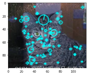
img = './cats_vs_dogs/train/cats/cat.1.jpg'
I = cv2.imread(img)
I = cv2.resize(I,(120,100))

FAST = cv2.FastFeatureDetector_create()
kps = FAST.detect(I, None)
cv2.drawKeypoints(I,kps,I,(0,255,255),flags=cv2.DRAW_MATCHES_FLAGS_DRAW_RICH_KEYPOINTS)
plt.imshow(I)
<matplotlib.image.AxesImage at 0x1af8c377370>
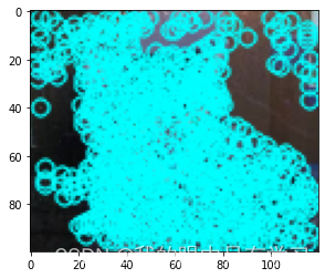
由此可见FAST方法的提取结果对背景噪点的敏感性并不强,于是我们这里选择SIFT作为我们的特征方案
查看特征矩阵
img = cv2.imread('./cats_vs_dogs/train/cats/cat.1.jpg')
img.shape
(280, 300, 3)
I = cv2.resize(img,(120,100))
I.shape
(100, 120, 3)
SIFT = cv2.xfeatures2d.SIFT_create()
(kps, features) = SIFT.detectAndCompute(img, None)
features.shape
(606, 128)
img=features.reshape(1,features.shape[0]*features.shape[1])
img.shape
(1, 77568)
img = cv2.imread('./cats_vs_dogs/train/cats/cat.21.jpg')
I = cv2.resize(img,(120,100))
SIFT = cv2.xfeatures2d.SIFT_create()
(kps, features) = SIFT.detectAndCompute(I, None)
features.shape
(156, 128)
针对输入不同的图形,输出的特征矩阵维度不一致的情况,
我们选择对特征矩阵进行标准化处理后,再使用PCA降维,最后再reshape处理
from sklearn.decomposition import PCA
from sklearn.preprocessing import StandardScaler

img = cv2.imread('./cats_vs_dogs/train/cats/cat.21.jpg')
I = cv2.resize(img,(100,120))
SIFT = cv2.xfeatures2d.SIFT_create()
(kps, features) = SIFT.detectAndCompute(I, None)
features.shape
(170, 128)
features.T.shape
(128, 170)
from sklearn.decomposition import PCA
from sklearn.preprocessing import StandardScaler

img = cv2.imread('./cats_vs_dogs/train/cats/cat.21.jpg')
I = cv2.resize(img,(100,120))
SIFT = cv2.xfeatures2d.SIFT_create()
(kps, features) = SIFT.detectAndCompute(I, None)
features = StandardScaler().fit_transform(features.T)
features = PCA(n_components = 20).fit_transform(features)
print(img.shape)
print(features.shape)
(499, 431, 3)
(128, 20)
from sklearn.decomposition import PCA
from sklearn.preprocessing import StandardScaler

img = cv2.imread('./cats_vs_dogs/train/cats/cat.1.jpg')
I = cv2.resize(img,(120,100))
SIFT = cv2.xfeatures2d.SIFT_create()
(kps, features) = SIFT.detectAndCompute(I, None)
features = StandardScaler().fit_transform(features.T)
features = PCA(n_components = 20).fit_transform(features)
print(img.shape)
print(features.shape)
(280, 300, 3)
(128, 20)
将提取出来的特征向量替换之前图形一维化结果并进行训练预测
import cv2 #opencv库,用于读取图片等操作
import numpy as np
import pandas as pd
from sklearn.preprocessing import StandardScaler #标准差标准化
from sklearn.svm import SVC                      #svm包中SVC用于分类
from sklearn.decomposition import PCA            #特征分解模块的PCA用于降维

def get_data(x,y,types):
    file_path='./cats_vs_dogs/'+types+'/' #设置文件路径(这里为当前目录下的ORL文件夹,type输入训练集或测试集)
    train_set = pd.DataFrame()     #将train_set转换成DataFrame类型
    target=[]                               #标签列表
    IMG_H = 120
    IMG_W = 100

    for i in ('cat','dog'):            #i用于遍历ORL文件夹中的2个文件夹
        print('Starting Get Data From '+ types + ': ' + i)
        for j in range(x,y):                #j用于遍历每个文件夹的对应的x到y-1的图片
            img = cv2.imread(file_path+i+'s/'+i+'.'+str(j)+'.jpg')
            img = cv2.resize(img,(IMG_W,IMG_H))
            SIFT = cv2.xfeatures2d.SIFT_create()
            (kps, features) = SIFT.detectAndCompute(img, None)
            if features.shape[0] < 20:  # 特征维度小于20,说明该图形代表性不强,则跳过
                continue
            else:
                features = StandardScaler().fit_transform(features.T)
                features = PCA(n_components = 20).fit_transform(features)
                img=features.reshape(1,features.shape[0]*features.shape[1]) #将读入的图片数据转换成一维
                img=pd.DataFrame(img)           #将一维的图片数据转成DataFrame类型
                train_set=pd.concat([train_set,img],axis=0)#按行拼接DataFrame矩阵
                target.append(i)                #读入标签(图片文件夹中的人脸是同一个类的)
#                 print('Get Data Finish ' + str(j))
    train_set.index=list(range(0,train_set.shape[0])) #设置 train_set的行索引
    target=pd.DataFrame(target)             #将标签列表转成DataFrame类型
    return train_set,target                 #返回数据集和标签

#1、获取数据
data_train,target_train=get_data(0,500,'train') #读取前500张图片为训练集
data_test,target_test=get_data(2000,2300,'validation')  #读取后200张图片为测试集
Starting Get Data From train:cat
Starting Get Data From train:dog
Starting Get Data From validation:cat
Starting Get Data From validation:dog
#2、数据标准化 标准差标准化
stdScaler = StandardScaler().fit(data_train)
trainStd = stdScaler.transform(data_train)
#stdScaler = StandardScaler().fit(data_test)
testStd = stdScaler.transform(data_test)
#3、PCA降维
pca = PCA(n_components=20).fit(trainStd)
trainStd = pca.transform(trainStd)
testStd = pca.transform(testStd)
trainStd.shape
(999, 20)
testStd.shape
(598, 20)
特征提取后进行训练预测
#4、建立SVM模型  默认为径向基核函数kernel='rbf' 多项式核函数kernel='poly'
#svm = SVC().fit(trainStd,target_train)
svm = SVC(kernel='poly').fit(trainStd,target_train)
print('建立的SVM模型为:\n',svm)
#4、预测训练集结果
target_pred = svm.predict(testStd)
print('预测前10个结果为:\n',target_pred[:10])
target_test=target_test.values    #Dataframe转ndarray方便后面准确率的判断
true=0
for i in range(0,200):
    if target_pred[i] == target_test[i]:
        true=true+1
print('预测对的结果数目为:', true)
print('预测错的的结果数目为:', target_test.shape[0]-true)
print('预测结果准确率为:', true/target_test.shape[0])
建立的SVM模型为:
 SVC(kernel='poly')
预测前10个结果为:
 ['cat' 'cat' 'cat' 'cat' 'cat' 'cat' 'cat' 'cat' 'cat' 'cat']
预测对的结果数目为: 154
预测错的的结果数目为: 444
预测结果准确率为: 0.25752508361204013
其他的机器学习算法
from sklearn import preprocessing

X_train = trainStd
y_train = target_train
X_test = testStd
y_test = target_test

# MultinomialNB的训练集数据不能为负
def min_max_normalization(np_array):
    min_max_scaler = preprocessing.MinMaxScaler()
    ret = min_max_scaler.fit_transform(np_array)
    return ret

X_train_unNegative = min_max_normalization(X_train)
X_test_unNegative = min_max_normalization(X_test)

#1.导入
from sklearn.naive_bayes import MultinomialNB
#2.创建模型
mNB = MultinomialNB()
#3.训练
mNB.fit(X_train_unNegative,y_train)
#4.预测
y_pre_MNB = mNB.predict(X_test_unNegative)

#1.导入
from sklearn.naive_bayes import GaussianNB
#2.创建模型
gNB = GaussianNB()
#3.训练
gNB.fit(X_train,y_train)
#4.预测
y_pre_gNB = gNB.predict(X_test)

#1.导入
from sklearn.neighbors import KNeighborsClassifier
#2.创建模型
knn = KNeighborsClassifier(n_neighbors=5)
#3.训练
knn.fit(X_train,y_train)
#4.预测
y_pre_knn = knn.predict(X_test)

#1.导入
from sklearn.linear_model import LogisticRegression
#2.创建模型
Logis = LogisticRegression(random_state=0)
#3.训练
Logis.fit(X_train,y_train)
#4.预测
y_pre_Log = Logis.predict(X_test)

#1.导入
from sklearn.tree import DecisionTreeClassifier
#2.创建模型
DT = DecisionTreeClassifier(max_depth=5)
#3.训练
DT.fit(X_train,y_train)
#4.预测
y_pre_DT = DT.predict(X_test)

#1.导入
from sklearn.linear_model import SGDClassifier
#2.创建模型
SGD = SGDClassifier(loss="hinge", penalty="l2")
#3.训练
SGD.fit(X_train,y_train)
#4.预测
y_pre_SGD = SGD.predict(X_test)

#1.导入
from sklearn.svm import SVC
#2.创建模型
SVC = SVC(C=1,kernel="rbf")
#3.训练
SVC.fit(X_train,y_train)
#4.预测
y_pre_SVC = SVC.predict(X_test)

#### 6.2.6 模型检验

import numpy as np
from sklearn.metrics import accuracy_score
from sklearn.metrics import classification_report

import warnings
warnings.filterwarnings("ignore")

print("---------------------------MNB-------------------------------")
print(classification_report(y_test, y_pre_MNB, target_names=['f','t']))
print("---------------------------gNB-------------------------------")
print(classification_report(y_test, y_pre_gNB, target_names=['f','t']))
print("---------------------------knn-------------------------------")
print(classification_report(y_test, y_pre_knn, target_names=['f','t']))
print("---------------------------Logstic---------------------------")
print(classification_report(y_test, y_pre_Log, target_names=['f','t']))
print("---------------------------DT--------------------------------")
print(classification_report(y_test, y_pre_DT, target_names=['f','t']))
print("---------------------------SGD-------------------------------")
print(classification_report(y_test, y_pre_SGD, target_names=['f','t']))
print("---------------------------SVC------------------------------")
print(classification_report(y_test, y_pre_SVC, target_names=['f','t']))
---------------------------MNB-------------------------------
              precision    recall  f1-score   support

           f       0.52      0.54      0.53       299
           t       0.52      0.50      0.51       299

    accuracy                           0.52       598
   macro avg       0.52      0.52      0.52       598
weighted avg       0.52      0.52      0.52       598

---------------------------gNB-------------------------------
              precision    recall  f1-score   support

           f       0.54      0.88      0.66       299
           t       0.66      0.24      0.35       299

    accuracy                           0.56       598
   macro avg       0.60      0.56      0.51       598
weighted avg       0.60      0.56      0.51       598

---------------------------knn-------------------------------
              precision    recall  f1-score   support

           f       0.53      0.76      0.62       299
           t       0.57      0.32      0.41       299

    accuracy                           0.54       598
   macro avg       0.55      0.54      0.51       598
weighted avg       0.55      0.54      0.51       598

---------------------------Logstic---------------------------
              precision    recall  f1-score   support

           f       0.56      0.59      0.57       299
           t       0.56      0.53      0.55       299

    accuracy                           0.56       598
   macro avg       0.56      0.56      0.56       598
weighted avg       0.56      0.56      0.56       598

---------------------------DT--------------------------------
              precision    recall  f1-score   support

           f       0.52      0.43      0.47       299
           t       0.51      0.60      0.55       299

    accuracy                           0.51       598
   macro avg       0.51      0.51      0.51       598
weighted avg       0.51      0.51      0.51       598

---------------------------SGD-------------------------------
              precision    recall  f1-score   support

           f       0.51      0.46      0.49       299
           t       0.51      0.56      0.53       299

    accuracy                           0.51       598
   macro avg       0.51      0.51      0.51       598
weighted avg       0.51      0.51      0.51       598

---------------------------SVC------------------------------
              precision    recall  f1-score   support

           f       0.55      0.72      0.62       299
           t       0.60      0.42      0.49       299

    accuracy                           0.57       598
   macro avg       0.57      0.57      0.56       598
weighted avg       0.57      0.57      0.56       598
效果精度都很一般,所以我们改为使用深度学习算法进行改进
深度学习方法(主要使用tensorflow和keras)
CNN
from __future__ import absolute_import, division, print_function, unicode_literals
#导入Tensorflow和构建模型所需的Keras类。
import tensorflow as tf
from tensorflow.keras.models import Sequential
from tensorflow.keras.layers import Dense, Conv2D, Flatten, Dropout, MaxPooling2D
from tensorflow.keras.preprocessing.image import ImageDataGenerator

import os
import numpy as np
import matplotlib.pyplot as plt


## 设置模型
batch_size = 128 # 8的倍数
epochs = 60 # 对每个batch 循环训练60次
IMG_HEIGHT = 224
IMG_WIDTH = 224
image_size = (IMG_WIDTH,IMG_HEIGHT)

# 生成训练集和测试集
train_image_generator = ImageDataGenerator(rescale=1./255) # 色素矩阵归一化(0~255—》0~1)
validation_image_generator = ImageDataGenerator(rescale=1./255) # 色素矩阵归一化(0~255—》0~1)

# 用预设好的生成器对我们的输入数据进行生成
train_data_gen = train_image_generator.flow_from_directory(batch_size=batch_size,
                                                           directory=train_dir,
                                                           shuffle=True,
                                                           target_size=(IMG_HEIGHT, IMG_WIDTH),
                                                           class_mode='binary')

val_data_gen = validation_image_generator.flow_from_directory(batch_size=batch_size,
                                                              directory=validation_dir,
                                                              target_size=(IMG_HEIGHT, IMG_WIDTH),
                                                              class_mode='binary')

sample_training_images, _ = next(train_data_gen)

# 预设的神经网络模型(层结构)
model = Sequential([
    Conv2D(16, 3, padding='same', activation='relu', input_shape=(IMG_HEIGHT, IMG_WIDTH ,3)),
    MaxPooling2D(),
    Conv2D(32, 3, padding='same', activation='relu'),
    MaxPooling2D(),
    Conv2D(64, 3, padding='same', activation='relu'),
    MaxPooling2D(),
    Flatten(),
    Dense(512, activation='relu'),
    Dense(1, activation='sigmoid')
])

# 预设损失函数和精准度指标
model.compile(optimizer='adam',
              loss='binary_crossentropy',
              metrics=['accuracy'])

# 训练过程输出
history = model.fit_generator(
    train_data_gen,
    steps_per_epoch=total_train // batch_size,
    epochs=epochs,
    validation_data=val_data_gen,
    validation_steps=total_val // batch_size
)
Found 1980 images belonging to 2 classes.
Found 1000 images belonging to 2 classes.
Epoch 1/60
15/15 [==============================] - 30s 2s/step - loss: 0.9818 - accuracy: 0.5065 - val_loss: 0.6921 - val_accuracy: 0.4989
Epoch 2/60
15/15 [==============================] - 33s 2s/step - loss: 0.6831 - accuracy: 0.5778 - val_loss: 0.6699 - val_accuracy: 0.6138
Epoch 3/60
15/15 [==============================] - 30s 2s/step - loss: 0.6553 - accuracy: 0.6145 - val_loss: 0.6615 - val_accuracy: 0.6295
Epoch 4/60
15/15 [==============================] - 31s 2s/step - loss: 0.6140 - accuracy: 0.6766 - val_loss: 0.6000 - val_accuracy: 0.6808
Epoch 5/60
15/15 [==============================] - 31s 2s/step - loss: 0.5479 - accuracy: 0.7219 - val_loss: 0.5935 - val_accuracy: 0.6875
Epoch 6/60
15/15 [==============================] - 29s 2s/step - loss: 0.4714 - accuracy: 0.7819 - val_loss: 0.6428 - val_accuracy: 0.6719
Epoch 7/60
15/15 [==============================] - 29s 2s/step - loss: 0.4090 - accuracy: 0.8197 - val_loss: 0.5610 - val_accuracy: 0.7266
Epoch 8/60
15/15 [==============================] - 28s 2s/step - loss: 0.3202 - accuracy: 0.8677 - val_loss: 0.6285 - val_accuracy: 0.7031
Epoch 9/60
15/15 [==============================] - 28s 2s/step - loss: 0.2445 - accuracy: 0.9136 - val_loss: 0.6724 - val_accuracy: 0.7109
Epoch 10/60
15/15 [==============================] - 28s 2s/step - loss: 0.1916 - accuracy: 0.9260 - val_loss: 0.7574 - val_accuracy: 0.7031
Epoch 11/60
15/15 [==============================] - 28s 2s/step - loss: 0.1450 - accuracy: 0.9519 - val_loss: 0.8262 - val_accuracy: 0.7087
Epoch 12/60
15/15 [==============================] - 28s 2s/step - loss: 0.0967 - accuracy: 0.9719 - val_loss: 1.0843 - val_accuracy: 0.6842
Epoch 13/60
15/15 [==============================] - 28s 2s/step - loss: 0.0701 - accuracy: 0.9833 - val_loss: 0.9894 - val_accuracy: 0.7042
Epoch 14/60
15/15 [==============================] - 28s 2s/step - loss: 0.0516 - accuracy: 0.9860 - val_loss: 1.1608 - val_accuracy: 0.6842
Epoch 15/60
15/15 [==============================] - 28s 2s/step - loss: 0.0355 - accuracy: 0.9930 - val_loss: 1.2195 - val_accuracy: 0.6964
Epoch 16/60
15/15 [==============================] - 29s 2s/step - loss: 0.0288 - accuracy: 0.9919 - val_loss: 1.2190 - val_accuracy: 0.7042
Epoch 17/60
15/15 [==============================] - 28s 2s/step - loss: 0.0221 - accuracy: 0.9968 - val_loss: 1.3021 - val_accuracy: 0.6931
Epoch 18/60
15/15 [==============================] - 28s 2s/step - loss: 0.0129 - accuracy: 0.9989 - val_loss: 1.3455 - val_accuracy: 0.7165
Epoch 19/60
15/15 [==============================] - 28s 2s/step - loss: 0.0086 - accuracy: 0.9995 - val_loss: 1.4737 - val_accuracy: 0.7188
Epoch 20/60
15/15 [==============================] - 28s 2s/step - loss: 0.0052 - accuracy: 1.0000 - val_loss: 1.5416 - val_accuracy: 0.7054
Epoch 21/60
15/15 [==============================] - 29s 2s/step - loss: 0.0029 - accuracy: 1.0000 - val_loss: 1.6283 - val_accuracy: 0.7132
Epoch 22/60
15/15 [==============================] - 28s 2s/step - loss: 0.0021 - accuracy: 1.0000 - val_loss: 1.6780 - val_accuracy: 0.7065
Epoch 23/60
15/15 [==============================] - 28s 2s/step - loss: 0.0016 - accuracy: 1.0000 - val_loss: 1.7875 - val_accuracy: 0.7009
Epoch 24/60
15/15 [==============================] - 28s 2s/step - loss: 0.0012 - accuracy: 1.0000 - val_loss: 1.8343 - val_accuracy: 0.7020
Epoch 25/60
15/15 [==============================] - 28s 2s/step - loss: 0.0010 - accuracy: 1.0000 - val_loss: 1.8416 - val_accuracy: 0.7098
Epoch 26/60
15/15 [==============================] - 28s 2s/step - loss: 8.8058e-04 - accuracy: 1.0000 - val_loss: 1.7859 - val_accuracy: 0.7098
Epoch 27/60
15/15 [==============================] - 28s 2s/step - loss: 7.7191e-04 - accuracy: 1.0000 - val_loss: 1.9306 - val_accuracy: 0.6953
Epoch 28/60
15/15 [==============================] - 28s 2s/step - loss: 6.4186e-04 - accuracy: 1.0000 - val_loss: 1.9015 - val_accuracy: 0.7109
Epoch 29/60
15/15 [==============================] - 28s 2s/step - loss: 6.0752e-04 - accuracy: 1.0000 - val_loss: 1.9456 - val_accuracy: 0.7009
Epoch 30/60
15/15 [==============================] - 28s 2s/step - loss: 5.6044e-04 - accuracy: 1.0000 - val_loss: 1.9393 - val_accuracy: 0.7098
Epoch 31/60
15/15 [==============================] - 28s 2s/step - loss: 5.0215e-04 - accuracy: 1.0000 - val_loss: 1.8479 - val_accuracy: 0.7165
Epoch 32/60
15/15 [==============================] - 28s 2s/step - loss: 4.5813e-04 - accuracy: 1.0000 - val_loss: 1.9279 - val_accuracy: 0.7154
Epoch 33/60
15/15 [==============================] - 28s 2s/step - loss: 3.9756e-04 - accuracy: 1.0000 - val_loss: 2.0915 - val_accuracy: 0.7054
Epoch 34/60
15/15 [==============================] - 28s 2s/step - loss: 3.6603e-04 - accuracy: 1.0000 - val_loss: 2.0736 - val_accuracy: 0.7176
Epoch 35/60
15/15 [==============================] - 28s 2s/step - loss: 3.2996e-04 - accuracy: 1.0000 - val_loss: 2.1025 - val_accuracy: 0.7098
Epoch 36/60
15/15 [==============================] - 28s 2s/step - loss: 3.0829e-04 - accuracy: 1.0000 - val_loss: 2.1845 - val_accuracy: 0.7054
Epoch 37/60
15/15 [==============================] - 28s 2s/step - loss: 2.9793e-04 - accuracy: 1.0000 - val_loss: 2.0831 - val_accuracy: 0.7165
Epoch 38/60
15/15 [==============================] - 31s 2s/step - loss: 2.5878e-04 - accuracy: 1.0000 - val_loss: 2.1099 - val_accuracy: 0.7210
Epoch 39/60
15/15 [==============================] - 28s 2s/step - loss: 2.4059e-04 - accuracy: 1.0000 - val_loss: 2.1404 - val_accuracy: 0.7087
Epoch 40/60
15/15 [==============================] - 28s 2s/step - loss: 2.1804e-04 - accuracy: 1.0000 - val_loss: 2.2382 - val_accuracy: 0.7076
Epoch 41/60
15/15 [==============================] - 28s 2s/step - loss: 2.0417e-04 - accuracy: 1.0000 - val_loss: 2.2357 - val_accuracy: 0.7054
Epoch 42/60
15/15 [==============================] - 28s 2s/step - loss: 1.9786e-04 - accuracy: 1.0000 - val_loss: 2.3309 - val_accuracy: 0.6953
Epoch 43/60
15/15 [==============================] - 28s 2s/step - loss: 1.7737e-04 - accuracy: 1.0000 - val_loss: 2.2356 - val_accuracy: 0.7121
Epoch 44/60
15/15 [==============================] - 28s 2s/step - loss: 1.6442e-04 - accuracy: 1.0000 - val_loss: 2.2920 - val_accuracy: 0.7121
Epoch 45/60
15/15 [==============================] - 28s 2s/step - loss: 1.5981e-04 - accuracy: 1.0000 - val_loss: 2.2364 - val_accuracy: 0.7243
Epoch 46/60
15/15 [==============================] - 29s 2s/step - loss: 1.4674e-04 - accuracy: 1.0000 - val_loss: 2.2769 - val_accuracy: 0.7154
Epoch 47/60
15/15 [==============================] - 28s 2s/step - loss: 1.4055e-04 - accuracy: 1.0000 - val_loss: 2.2786 - val_accuracy: 0.7121
Epoch 48/60
15/15 [==============================] - 28s 2s/step - loss: 1.3360e-04 - accuracy: 1.0000 - val_loss: 2.3075 - val_accuracy: 0.7076
Epoch 49/60
15/15 [==============================] - 28s 2s/step - loss: 1.2415e-04 - accuracy: 1.0000 - val_loss: 2.3485 - val_accuracy: 0.7042
Epoch 50/60
15/15 [==============================] - 28s 2s/step - loss: 1.2083e-04 - accuracy: 1.0000 - val_loss: 2.4608 - val_accuracy: 0.7087
Epoch 51/60
15/15 [==============================] - 28s 2s/step - loss: 1.0913e-04 - accuracy: 1.0000 - val_loss: 2.4066 - val_accuracy: 0.7098
Epoch 52/60
15/15 [==============================] - 28s 2s/step - loss: 1.0328e-04 - accuracy: 1.0000 - val_loss: 2.3571 - val_accuracy: 0.7098
Epoch 53/60
15/15 [==============================] - 28s 2s/step - loss: 9.9703e-05 - accuracy: 1.0000 - val_loss: 2.3991 - val_accuracy: 0.7165
Epoch 54/60
15/15 [==============================] - 28s 2s/step - loss: 9.5948e-05 - accuracy: 1.0000 - val_loss: 2.4797 - val_accuracy: 0.7042
Epoch 55/60
15/15 [==============================] - 28s 2s/step - loss: 9.2920e-05 - accuracy: 1.0000 - val_loss: 2.3754 - val_accuracy: 0.7143
Epoch 56/60
15/15 [==============================] - 28s 2s/step - loss: 8.4558e-05 - accuracy: 1.0000 - val_loss: 2.4235 - val_accuracy: 0.7154
Epoch 57/60
15/15 [==============================] - 28s 2s/step - loss: 8.2813e-05 - accuracy: 1.0000 - val_loss: 2.5078 - val_accuracy: 0.7109
Epoch 58/60
15/15 [==============================] - 28s 2s/step - loss: 7.8685e-05 - accuracy: 1.0000 - val_loss: 2.4555 - val_accuracy: 0.7154
Epoch 59/60
15/15 [==============================] - 28s 2s/step - loss: 7.3389e-05 - accuracy: 1.0000 - val_loss: 2.5217 - val_accuracy: 0.7020
Epoch 60/60
15/15 [==============================] - 28s 2s/step - loss: 7.1709e-05 - accuracy: 1.0000 - val_loss: 2.4298 - val_accuracy: 0.7165
print(model.summary())
Model: "sequential"
_________________________________________________________________
Layer (type)                 Output Shape              Param #
=================================================================
conv2d (Conv2D)              (None, 224, 224, 16)      448
_________________________________________________________________
max_pooling2d (MaxPooling2D) (None, 112, 112, 16)      0
_________________________________________________________________
conv2d_1 (Conv2D)            (None, 112, 112, 32)      4640
_________________________________________________________________
max_pooling2d_1 (MaxPooling2 (None, 56, 56, 32)        0
_________________________________________________________________
conv2d_2 (Conv2D)            (None, 56, 56, 64)        18496
_________________________________________________________________
max_pooling2d_2 (MaxPooling2 (None, 28, 28, 64)        0
_________________________________________________________________
flatten (Flatten)            (None, 50176)             0
_________________________________________________________________
dense_14 (Dense)             (None, 512)               25690624
_________________________________________________________________
dense_15 (Dense)             (None, 1)                 513
=================================================================
Total params: 25,714,721
Trainable params: 25,714,721
Non-trainable params: 0
_________________________________________________________________
None
acc = history.history['accuracy']
val_acc = history.history['val_accuracy']

loss = history.history['loss']
val_loss = history.history['val_loss']

epochs_range = range(epochs)

plt.figure(figsize=(10, 8))
plt.subplot(1, 2, 1)
plt.plot(epochs_range, acc, label='Training Accuracy')
plt.plot(epochs_range, val_acc, label='Validation Accuracy')
plt.legend(loc='lower right')
plt.title('Training VS Validation Accuracy')

plt.subplot(1, 2, 2)
plt.plot(epochs_range, loss, label='Training Loss')
plt.plot(epochs_range, val_loss, label='Validation Loss')
plt.legend(loc='upper right')
plt.title('Training and Validation Loss')
plt.show()
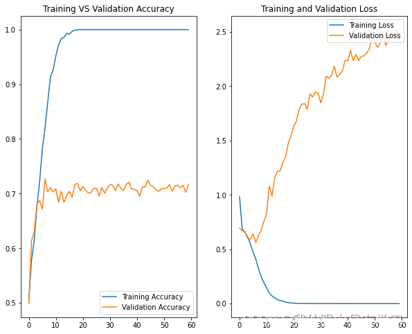
# 实例检测

from keras.preprocessing import image
from tensorflow.keras.applications.resnet50 import preprocess_input

images = []
path='./test/'
for f in os.listdir(path):
    img = image.load_img(path + f, target_size=image_size)
    img_array = image.img_to_array(img)

    x = np.expand_dims(img_array, axis=0)
    x = preprocess_input(x)
    predict_x=model.predict(x)
    classes_x=int(predict_x[0][0])
# 其中猫为0,狗为1
    print(f,classes_x)
cat.png 0
cat (2).png 0
dog.2002.jpg 1
dog.8.jpg 0
dog.9.jpg 0
dog.10.jpg 1
dog.11.jpg 1
dog.12.jpg 0
dog.13.jpg 0
dog.104.jpg 0
dog.105.jpg 1
dog.106.jpg 1
dog.107.jpg 1
dog.108.jpg 0
dog.109.jpg 1
dog.110.jpg 1
dog.111.jpg 1
dog.112.jpg 1
dog.113.jpg 1
dog.114.jpg 0
dog.115.jpg 0
Kaggle用户TIFOSI528 模型Loss约0.053
因为效果都一般,所以我们选择从网上借鉴一下kaggle竞赛历年cat vs dog的冠军模型进行预测
GitHub-Link:https://github.com/TIFOSI528/dogs-vs-cats
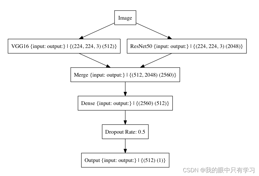
数据增强
# 计算每张图片的颜色/像素比率,并保存到比率列表中

from PIL import Image
import os
import numpy as np
import shutil
from collections import Counter

for i in ('cats','dogs'):
    ratio_list = []
    targetnames = os.listdir('./cats_vs_dogs/train/'+i+'/')
    for name in targetnames[1:]:
        im = Image.open('./cats_vs_dogs/train/'+i+'/'+name)
        x = im.histogram(mask=None)
        count = Counter(x)
        ratio_list.append(float(len(count))/len(x))
    q99,q01 = np.percentile(ratio_list, [99, 1])
    print('calculate the percentile [99, 1] of ratio_list_'+ i +'  '+'q99:'+str(q99)+',   q01:'+str(q01))
calculate the percentile [99, 1] of ratio_list_cats  q99:0.8008072916666666,   q01:0.20174479166666667
calculate the percentile [99, 1] of ratio_list_dogs  q99:0.8086197916666666,   q01:0.1925260416666667
ratio_list_cats = [0.8008,0.2017]
ratio_list_dogs = [0.8086,0.1925]
# 找图片 "颜色/像素比率小于 q01"

from keras.preprocessing.image import img_to_array, load_img
import shutil
import os
import matplotlib.pyplot as plt

dogs_outline_list = []
cats_outline_list = []

for i in ('cats','dogs'):
    targetnames = os.listdir('./cats_vs_dogs/train/'+i+'/')
    for name in targetnames[:]:
        im = Image.open('./cats_vs_dogs/train/'+i+'/'+name)
        x = im.histogram(mask=None)
        count = Counter(x)
        if i == 'cats':
            if float(len(count))/len(x) < ratio_list_cats[1]:
                cats_outline_list.append(name)
        else:
            if float(len(count))/len(x) < ratio_list_dogs[1]:
                dogs_outline_list.append(name)
cats_outline_list
['cat.146.jpg',
 'cat.183.jpg',
 'cat.273.jpg',
 'cat.44.jpg',
 'cat.48.jpg',
 'cat.485.jpg',
 'cat.575.jpg',
 'cat.596.jpg',
 'cat.664.jpg',
 'cat.862.jpg']
dogs_outline_list
['dog.12.jpg',
 'dog.284.jpg',
 'dog.296.jpg',
 'dog.531.jpg',
 'dog.561.jpg',
 'dog.630.jpg',
 'dog.881.jpg',
 'dog.927.jpg',
 'dog.943.jpg',
 'dog.990.jpg']
for i in ('cats','dogs'):
    targetnames = os.listdir('./cats_vs_dogs/train/'+i+'/')
    if i =='cats':
        for name in cats_outline_list:
            shutil.move('./cats_vs_dogs/train/'+i+'/'+ name, './cats_vs_dogs/outline/'+i+'/'+ name)
    else:
        for name in dogs_outline_list:
            shutil.move('./cats_vs_dogs/train/'+i+'/'+ name, './cats_vs_dogs/outline/'+i+'/'+ name)
预测
利用pre-trained神经网络(VGG16 & ResNet50)对图像进行特征提取
# train the FC layer by Adadelta before fine-tuning, and save the weights as TL_VGG_Res_13.h5

import keras
from tensorflow.keras.applications.vgg16 import VGG16
from tensorflow.keras.applications.resnet50 import ResNet50
from tensorflow.keras.applications.imagenet_utils import preprocess_input
from keras.models import Model
from keras.layers import *
from tensorflow.keras.optimizers import Adadelta
from keras.preprocessing.image import ImageDataGenerator
import h5py


heights = 224
widths = 224
batch_size = 16
epochs = 10

input_tensor = Input((heights, widths, 3))
x = input_tensor
base_model1 = VGG16(input_tensor=x, weights='imagenet', include_top=False)
base_model2 = ResNet50(input_tensor=x, weights='imagenet', include_top=False)

x1 = base_model1.output
x2 = base_model2.output

x1 = GlobalAveragePooling2D()(x1)
x2 = GlobalAveragePooling2D()(x2)

x = keras.layers.concatenate([x1, x2])

x = Dense(512, activation='relu')(x)
x = Dropout(0.5)(x)

predictions = Dense(1, activation='sigmoid')(x)

model = Model(inputs=input_tensor, outputs=predictions)

for layer in base_model1.layers[:]:
    layer.trainable = False

for layer in base_model2.layers[:]:
    layer.trainable = False

model.summary()


# prepare data augmentation configuration

def preprocess_input_new(x):

    X = np.expand_dims(x, axis=0)
    X = preprocess_input(X)
    return X[0]

batch_size = 16
train_datagen = ImageDataGenerator(
        shear_range=0.2,
        zoom_range=0.2,
        fill_mode='nearest',
        horizontal_flip=True,
        rotation_range = 30,
        preprocessing_function=preprocess_input_new
)

validation_datagen = ImageDataGenerator(preprocessing_function=preprocess_input_new)

train_generator = train_datagen.flow_from_directory(
    './cats_vs_dogs/train/',
    target_size=(heights, widths),
    batch_size=batch_size,
    class_mode='binary',
)


validation_generator = validation_datagen.flow_from_directory(
    './cats_vs_dogs/validation/',
    target_size=(heights, widths),
    batch_size=batch_size,
    class_mode='binary',
    )

#sgd = SGD(lr=1e-4, momentum=0.9, nesterov=True)

model.compile(optimizer = 'adadelta', loss='binary_crossentropy', metrics=['accuracy'])

#model.load_weights('TL_VGG_Res_3.h5')

history = model.fit_generator(
    train_generator,
    epochs = epochs,
    steps_per_epoch = 1980/batch_size,
    validation_data = validation_generator, validation_steps = 1000/batch_size)

#json_string = model.to_json()
#open('TL_VGG16_model_architecture_1.json','w').write(json_string)
model.save_weights('TL_VGG_Res_13.h5')
Model: "model_3"
__________________________________________________________________________________________________
Layer (type)                    Output Shape         Param #     Connected to
==================================================================================================
input_4 (InputLayer)            [(None, 224, 224, 3) 0
__________________________________________________________________________________________________
conv1_pad (ZeroPadding2D)       (None, 230, 230, 3)  0           input_4[0][0]
__________________________________________________________________________________________________
conv1_conv (Conv2D)             (None, 112, 112, 64) 9472        conv1_pad[0][0]
__________________________________________________________________________________________________
conv1_bn (BatchNormalization)   (None, 112, 112, 64) 256         conv1_conv[0][0]
__________________________________________________________________________________________________
conv1_relu (Activation)         (None, 112, 112, 64) 0           conv1_bn[0][0]
__________________________________________________________________________________________________
pool1_pad (ZeroPadding2D)       (None, 114, 114, 64) 0           conv1_relu[0][0]
__________________________________________________________________________________________________
pool1_pool (MaxPooling2D)       (None, 56, 56, 64)   0           pool1_pad[0][0]
__________________________________________________________________________________________________
conv2_block1_1_conv (Conv2D)    (None, 56, 56, 64)   4160        pool1_pool[0][0]
__________________________________________________________________________________________________
conv2_block1_1_bn (BatchNormali (None, 56, 56, 64)   256         conv2_block1_1_conv[0][0]
__________________________________________________________________________________________________
···
==================================================================================================
Total params: 39,614,145
Trainable params: 1,311,745
Non-trainable params: 38,302,400
__________________________________________________________________________________________________
Found 1980 images belonging to 2 classes.
Found 1000 images belonging to 2 classes.
Epoch 1/10
123/123 [==============================] - 371s 3s/step - loss: 2.2716 - accuracy: 0.4884 - val_loss: 1.7579 - val_accuracy: 0.5060
Epoch 2/10
123/123 [==============================] - 371s 3s/step - loss: 1.4676 - accuracy: 0.5273 - val_loss: 1.1657 - val_accuracy: 0.5630
Epoch 3/10
123/123 [==============================] - 369s 3s/step - loss: 1.3310 - accuracy: 0.5576 - val_loss: 0.8661 - val_accuracy: 0.6360
Epoch 4/10
123/123 [==============================] - 364s 3s/step - loss: 1.1553 - accuracy: 0.5965 - val_loss: 0.6890 - val_accuracy: 0.6870
Epoch 5/10
123/123 [==============================] - 366s 3s/step - loss: 1.0561 - accuracy: 0.6222 - val_loss: 0.5603 - val_accuracy: 0.7510
Epoch 6/10
123/123 [==============================] - 369s 3s/step - loss: 0.9314 - accuracy: 0.6586 - val_loss: 0.4693 - val_accuracy: 0.7930
Epoch 7/10
123/123 [==============================] - 371s 3s/step - loss: 0.8391 - accuracy: 0.6803 - val_loss: 0.3984 - val_accuracy: 0.8330
Epoch 8/10
123/123 [==============================] - 377s 3s/step - loss: 0.7245 - accuracy: 0.7192 - val_loss: 0.3498 - val_accuracy: 0.8560
Epoch 9/10
123/123 [==============================] - 374s 3s/step - loss: 0.7180 - accuracy: 0.7328 - val_loss: 0.3016 - val_accuracy: 0.8820
Epoch 10/10
123/123 [==============================] - 374s 3s/step - loss: 0.6513 - accuracy: 0.7444 - val_loss: 0.2653 - val_accuracy: 0.9010
# visualize the training process

import matplotlib.pyplot as plt

# list the data in history
print(history.history.keys())

# summarize history of accuracy
plt.plot(history.history['accuracy'])
plt.plot(history.history['val_accuracy'])
plt.title('model accuracy')
plt.ylabel('accuracy')
plt.xlabel('epoch')
plt.legend(['test', 'train'], loc='upper left')
plt.show()

# summarize history of loss
plt.plot(history.history['accuracy'])
plt.plot(history.history['val_loss'])
plt.title('model loss')
plt.ylabel('loss')
plt.xlabel('epoch')
plt.legend(['test', 'train'], loc='upper left')
plt.show()
dict_keys(['loss', 'accuracy', 'val_loss', 'val_accuracy'])
[外链图片转存失败,源站可能有防盗链机制,建议将图片保存下来直接上传(img-mE2mST6U-1663820520243)(output_57_1.png)]
[外链图片转存失败,源站可能有防盗链机制,建议将图片保存下来直接上传(img-LT6pRHPf-1663820520244)(output_57_2.png)]
再将提取得到的特征向量作为输入来训练一个新的全连接神经网络,以处理“猫狗”分类问题
# load the weight "TL_VGG_Res_13.h5", and fine-tune the last layers of VGG16 and ResNet50

import keras
from tensorflow.keras.applications.vgg16 import VGG16
from tensorflow.keras.applications.resnet50 import ResNet50
from tensorflow.keras.applications.imagenet_utils import preprocess_input
from tensorflow.keras.models import Model
from tensorflow.keras.layers import *
from tensorflow.keras.optimizers import SGD
from tensorflow.keras.optimizers import Adadelta
from keras.preprocessing.image import ImageDataGenerator
import h5py


heights = 224
widths = 224
batch_size = 8
epochs = 10

input_tensor = Input((heights, widths, 3))
x = input_tensor
base_model1 = VGG16(input_tensor=x, weights='imagenet', include_top=False)
base_model2 = ResNet50(input_tensor=x, weights='imagenet', include_top=False)

x1 = base_model1.output
x2 = base_model2.output

x1 = GlobalAveragePooling2D()(x1)
x2 = GlobalAveragePooling2D()(x2)

x = keras.layers.concatenate([x1, x2])

x = Dense(512, activation='relu')(x)
x = Dropout(0.5)(x)

predictions = Dense(1, activation='sigmoid')(x)

model = Model(inputs=input_tensor, outputs=predictions)

for layer in base_model1.layers[0:15]:
    layer.trainable = False

for layer in base_model2.layers[0:-10]:
    layer.trainable = False

model.summary()


# prepare data augmentation configuration

def preprocess_input_new(x):

    X = np.expand_dims(x, axis=0)
    X = preprocess_input(X)
    return X[0]

batch_size = 8
train_datagen = ImageDataGenerator(
        shear_range=0.2,
        zoom_range=0.2,
        fill_mode='nearest',
        horizontal_flip=True,
        rotation_range = 30,
        preprocessing_function=preprocess_input_new
)

validation_datagen = ImageDataGenerator(preprocessing_function=preprocess_input_new)

train_generator = train_datagen.flow_from_directory(
    './cats_vs_dogs/train/',
    target_size=(heights, widths),
    batch_size=batch_size,
    class_mode='binary',
)


validation_generator = validation_datagen.flow_from_directory(
    './cats_vs_dogs/validation/',
    target_size=(heights, widths),
    batch_size=batch_size,
    class_mode='binary',
    )

#we need to use SGD with a lower learning rate to fine-tune the model
sgd = SGD(lr=1e-4, momentum=0.9, nesterov=True)

model.compile(optimizer = sgd, loss='binary_crossentropy', metrics=['accuracy'])

#load the weights trained before
model.load_weights('TL_VGG_Res_13.h5')

history = model.fit_generator(
    train_generator,
    epochs = epochs,
    steps_per_epoch = 1980/batch_size,
    validation_data = validation_generator, validation_steps = 1000/batch_size)

#json_string = model.to_json()
#open('TL_VGG16_model_architecture_1.json','w').write(json_string)
model.save_weights('TL_VGG_Res_14.h5')
Model: "model_6"
__________________________________________________________________________________________________
Layer (type)                    Output Shape         Param #     Connected to
==================================================================================================
input_7 (InputLayer)            [(None, 224, 224, 3) 0
__________________________________________________________________________________________________
conv1_pad (ZeroPadding2D)       (None, 230, 230, 3)  0           input_7[0][0]
__________________________________________________________________________________________________
conv1_conv (Conv2D)             (None, 112, 112, 64) 9472        conv1_pad[0][0]
__________________________________________________________________________________________________
conv1_bn (BatchNormalization)   (None, 112, 112, 64) 256         conv1_conv[0][0]
__________________________________________________________________________________________________
conv1_relu (Activation)         (None, 112, 112, 64) 0           conv1_bn[0][0]
__________________________________________________________________________________________________
pool1_pad (ZeroPadding2D)       (None, 114, 114, 64) 0           conv1_relu[0][0]
__________________________________________________________________________________________________
pool1_pool (MaxPooling2D)       (None, 56, 56, 64)   0           pool1_pad[0][0]
__________________________________________________________________________________________________
···
==================================================================================================
Total params: 39,614,145
Trainable params: 12,856,833
Non-trainable params: 26,757,312
__________________________________________________________________________________________________
Found 1980 images belonging to 2 classes.
Found 1000 images belonging to 2 classes.
Epoch 1/10
247/247 [==============================] - 441s 2s/step - loss: 0.1623 - accuracy: 0.9348 - val_loss: 0.0342 - val_accuracy: 0.9840
Epoch 2/10
247/247 [==============================] - 431s 2s/step - loss: 0.0788 - accuracy: 0.9667 - val_loss: 0.0299 - val_accuracy: 0.9870
Epoch 3/10
247/247 [==============================] - 446s 2s/step - loss: 0.0446 - accuracy: 0.9803 - val_loss: 0.0312 - val_accuracy: 0.9890
Epoch 4/10
247/247 [==============================] - 444s 2s/step - loss: 0.0379 - accuracy: 0.9854 - val_loss: 0.0459 - val_accuracy: 0.9850
Epoch 5/10
247/247 [==============================] - 451s 2s/step - loss: 0.0441 - accuracy: 0.9833 - val_loss: 0.0290 - val_accuracy: 0.9880
Epoch 6/10
247/247 [==============================] - 451s 2s/step - loss: 0.0334 - accuracy: 0.9879 - val_loss: 0.0357 - val_accuracy: 0.9840
Epoch 7/10
247/247 [==============================] - 458s 2s/step - loss: 0.0208 - accuracy: 0.9924 - val_loss: 0.0558 - val_accuracy: 0.9820
Epoch 8/10
247/247 [==============================] - 447s 2s/step - loss: 0.0252 - accuracy: 0.9919 - val_loss: 0.0329 - val_accuracy: 0.9900
Epoch 9/10
247/247 [==============================] - 448s 2s/step - loss: 0.0198 - accuracy: 0.9934 - val_loss: 0.0448 - val_accuracy: 0.9860
Epoch 10/10
247/247 [==============================] - 441s 2s/step - loss: 0.0126 - accuracy: 0.9960 - val_loss: 0.0325 - val_accuracy: 0.9890
# visualize the training process

import matplotlib.pyplot as plt

# list the data in history
print(history.history.keys())

# summarize history of accuracy
plt.plot(history.history['accuracy'])
plt.plot(history.history['val_accuracy'])
plt.title('model accuracy')
plt.ylabel('accuracy')
plt.xlabel('epoch')
plt.legend(['test', 'train'], loc='upper left')
plt.show()

# summarize history of loss
plt.plot(history.history['loss'])
plt.plot(history.history['val_loss'])
plt.title('model loss')
plt.ylabel('loss')
plt.xlabel('epoch')
plt.legend(['test', 'train'], loc='upper left')
plt.show()
dict_keys(['loss', 'accuracy', 'val_loss', 'val_accuracy'])
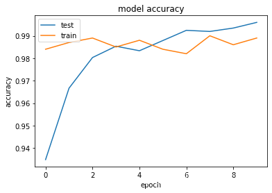
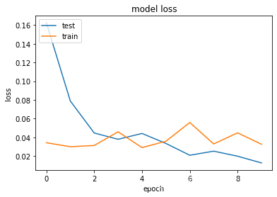


 16万+
16万+

 被折叠的 条评论
为什么被折叠?
被折叠的 条评论
为什么被折叠?
 到【灌水乐园】发言


