机器学习：逻辑回归--下采样

目录

前言

一、为什么使用下采样

1.例如：

2.导致：

3.办法：

4.结果：

二、代码实现

1.完整代码

2.导入库

3.可视化混淆矩阵

4.导入数据

5数据预处理

6.下采样

7.取出训练集和测试集

8.建立模型

9.进行测试

总结

---

前言

        下采样（Downsampling）是一种在数据处理中减少样本数量的技术。这种方法通常用于减少数据集的大小，以便进行更高效的计算或处理。下采样可以应用于不同类型的数据，包括信号、图像和分类数据。 

 

一、为什么使用下采样

• creditcard（点击这里下载文件）
• 有时我们的标签数据两极分化太严重

1.例如：

        标签为0的数据28w条，为1的数据只有400多条

 

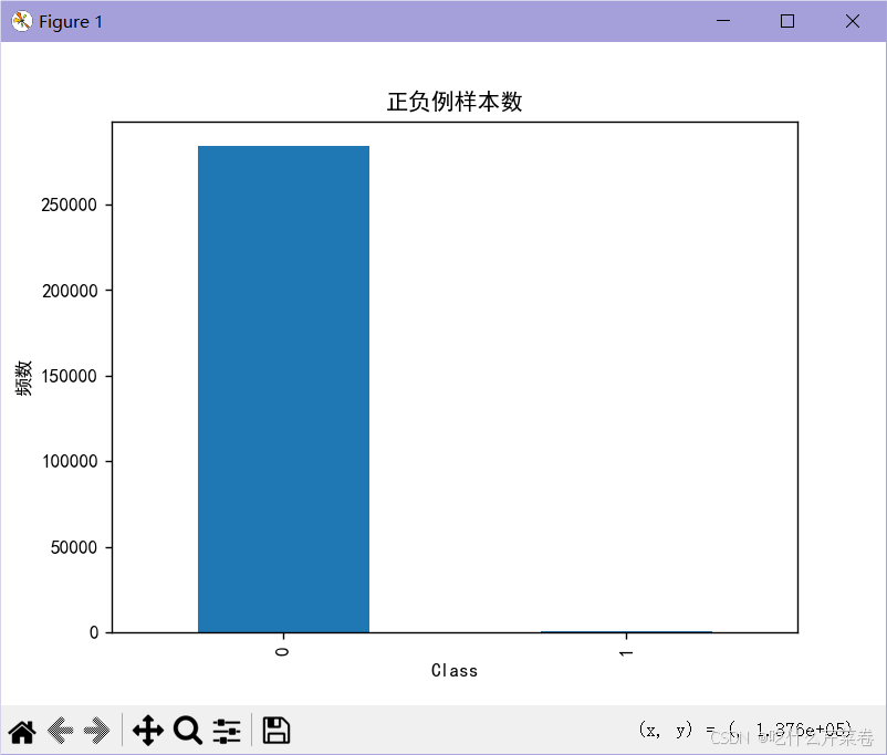
2.导致：

        这样训练出来的模型，使用测试集进行测试之后，对不同真实值的数据预测的结果差别很大，那么这个模型也就是一个不可用的模型

 

3.办法：

这时就需要使用下采样方法：

• 从数据量多的标签数据里随机选择与数据量少的标签数据等量的数据，并组合成小数据集

 

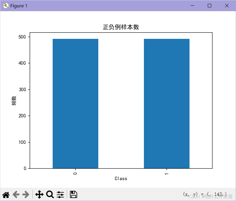
4.结果：

使用下采样训练模型之后，测试集的召回率有了很大提高。

 

 

二、代码实现

1.完整代码

import pandas as pd
import matplotlib.pyplot as plt
import numpy as np


# 可视化混淆矩阵
def cm_plot(y, yp):
    from sklearn.metrics import confusion_matrix
    import matplotlib.pyplot as plt

    cm = confusion_matrix(y, yp)
    plt.matshow(cm, cmap=plt.cm.Blues)
    plt.colorbar()
    for x in range(len(cm)):
        for y in range(len(cm)):
            plt.annotate(cm[x, y], xy=(y, x), horizontalalignment='center',
                         verticalalignment='center')
            plt.ylabel('True label')
            plt.xlabel('Predicted label')
    return plt

# 导入数据
data = pd.read_csv("creditcard.csv")

# 数据标准化: Z标准化
from sklearn.preprocessing import StandardScaler  # 可对多列进行标准化

scaler = StandardScaler()
a = data[['Amount']]  # 取出来变成df数据 因为fit_transform()需要传入df数据
data['Amount'] = scaler.fit_transform(a)  # 对Amount列数据进行标准化
data = data.drop(['Time'], axis=1)  # 删除无用列

"""下采样"""
positive_eg = data[data['Class'] == 0]
negative_eg = data[data['Class'] == 1]
np.random.seed(seed=22)  # 随机种子
positive_eg = positive_eg.sample(len(negative_eg))  # 从标签为0的样本中随机抽取与标签1数量相同的样本
data_c = pd.concat([positive_eg, negative_eg])  # 拼接数据 成为小数据集

plt.rcParams['font.sans-serif'] = ['SimHei']  # 设置字体
plt.rcParams['axes.unicode_minus'] = False  # 解决符号显示为方块的问题
labels_count = pd.value_counts(data_c['Class'])  # 统计0有多少个数据，1有多个数据
plt.title("正负例样本数")
plt.xlabel("类别")
plt.ylabel("频数")
labels_count.plot(kind='bar')  # 生成一个条形图，展示每个类别的样本数量。
plt.show()

# 随机取数据
from sklearn.model_selection import train_test_split

# 从小数据集中取出训练集和测试集
x_c = data_c.drop('Class', axis=1)
y_c = data_c.Class
x_c_train, x_c_test, y_c_train, y_c_test = \
    train_test_split(x_c, y_c, test_size=0.3, random_state=0)  # 随机取数据

# 从大数据集里取出训练集和测试集
x_w = data.drop('Class', axis=1)
y_w = data.Class
x_w_train, x_w_test, y_w_train, y_w_test = \
    train_test_split(x_w, y_w, test_size=0.3, random_state=0)  # 随机取数据

# 交叉验证选择较优惩罚因子 λ
from sklearn.model_selection import cross_val_score  # 交叉验证的函数
from sklearn.linear_model import LogisticRegression

# k折交叉验证选择C参数   使用小数据集
scores = []
c_param_range = [0.01, 0.1, 1, 10, 100]  # 待选C参数
for i in c_param_range:
    lr = LogisticRegression(C=i, penalty='l2', solver='lbfgs', max_iter=1000)  # 创建逻辑回归模型  lbfgs 拟牛顿法
    score = cross_val_score(lr, x_c_train, y_c_train, cv=8, scoring='recall')  # k折交叉验证 比较召回率
    score_mean = sum(score) / len(score)
    scores.append(score_mean)
    # print(score_mean)

best_c = c_param_range[np.argmax(scores)]  # 寻找到scores中最大值的对应的C参数
print(f"最优惩罚因子为:{best_c}")

# 建立最优模型  使用小数据集训练模型
lr = LogisticRegression(C=best_c, penalty='l2', max_iter=1000)
lr.fit(x_c_train, y_c_train)

"""绘制混淆矩阵"""
from sklearn import metrics

# 使用小数据集的训练集进行出厂前测试
train_predicted = lr.predict(x_c_train)  # 训练集特征数据x的预测值
# print(metrics.classification_report(y_c_train, train_predicted))  # 传入训练集真实的结果数据 与预测值组成矩阵
# cm_plot(y_train, train_predicted).show()   # 可视化混淆矩阵

# 使用小数据集的训练集进行测试
test_predicted = lr.predict(x_c_test)
# print(metrics.classification_report(y_c_test, test_predicted))
# cm_plot(y_test, test_predicted).show()

# 使用大数据集进行测试
w_test_predicted = lr.predict(x_w_test)
print(metrics.classification_report(y_w_test, w_test_predicted))

# 设置阈值  比较每个阈值的召回率 选出最优阈值  测试模型的阈值 用小数据集的测试集
thresholds = [0.1, 0.2, 0.3, 0.4, 0.5, 0.6, 0.7, 0.8, 0.9]
recalls = []
for i in thresholds:
    y_predict_proba = lr.predict_proba(x_w_test)  # 每条数据分类的预测概率
    y_predict_proba = pd.DataFrame(y_predict_proba)
    y_predict_proba = y_predict_proba.drop([0], axis=1)  # axis=1 表示删除列而不是行 与下面两行代码联动
    y_predict_proba[y_predict_proba[[1]] > i] = 1  # 数据大于i即判断为1类 人为设置阈值
    y_predict_proba[y_predict_proba[[1]] <= i] = 0
    a = y_predict_proba[y_predict_proba[1] > i]
    # cm_plot(y_w_test, y_predict_proba[1]).show()
    recall = metrics.recall_score(y_w_test, y_predict_proba[1])  # 计算召回率
    recalls.append(recall)
    print(f"{i} Recall metric in the testing dataset: {recall:.3f}")

 

2.导入库

import pandas as pd
import matplotlib.pyplot as plt
import numpy as np

 

3.可视化混淆矩阵

• 这是通用代码

# 可视化混淆矩阵
def cm_plot(y, yp):
    from sklearn.metrics import confusion_matrix
    import matplotlib.pyplot as plt

    cm = confusion_matrix(y, yp)
    plt.matshow(cm, cmap=plt.cm.Blues)
    plt.colorbar()
    for x in range(len(cm)):
        for y in range(len(cm)):
            plt.annotate(cm[x, y], xy=(y, x), horizontalalignment='center',
                         verticalalignment='center')
            plt.ylabel('True label')
            plt.xlabel('Predicted label')
    return plt

 

4.导入数据

# 导入数据
data = pd.read_csv("creditcard.csv")

 

5数据预处理

• 对特征数据进行标准化
• 去除无用数据

# 数据标准化: Z标准化
from sklearn.preprocessing import StandardScaler  # 可对多列进行标准化

scaler = StandardScaler()
a = data[['Amount']]  # 取出来变成df数据 因为fit_transform()需要传入df数据
data['Amount'] = scaler.fit_transform(a)  # 对Amount列数据进行标准化
data = data.drop(['Time'], axis=1)  # 删除无用列

 

6.下采样

• 分别取出各标签的数据
• 随机种子可以保证每一次取出来的随机数据是固定的
• 使用sample函数进行下采样操作
• 拼接数据 组成小数据集
• 绘制各标签数据条形图

"""下采样"""
positive_eg = data[data['Class'] == 0]
negative_eg = data[data['Class'] == 1]
np.random.seed(seed=22)  # 随机种子
positive_eg = positive_eg.sample(len(negative_eg))  # 从标签为0的样本中随机抽取与标签1数量相同的样本
data_c = pd.concat([positive_eg, negative_eg])  # 拼接数据 成为小数据集

plt.rcParams['font.sans-serif'] = ['SimHei']  # 设置字体
plt.rcParams['axes.unicode_minus'] = False  # 解决符号显示为方块的问题
labels_count = pd.value_counts(data_c['Class'])  # 统计0有多少个数据，1有多个数据
plt.title("正负例样本数")
plt.xlabel("类别")
plt.ylabel("频数")
labels_count.plot(kind='bar')  # 生成一个条形图，展示每个类别的样本数量。
plt.show()

 

7.取出训练集和测试集

• 分别取出小数据集和大数据集的训练集和测试集

# 随机取数据
from sklearn.model_selection import train_test_split

# 从小数据集中取出训练集和测试集
x_c = data_c.drop('Class', axis=1)
y_c = data_c.Class
x_c_train, x_c_test, y_c_train, y_c_test = \
    train_test_split(x_c, y_c, test_size=0.3, random_state=0)  # 随机取数据

# 从大数据集里取出训练集和测试集
x_w = data.drop('Class', axis=1)
y_w = data.Class
x_w_train, x_w_test, y_w_train, y_w_test = \
    train_test_split(x_w, y_w, test_size=0.3, random_state=0)  # 随机取数据

 

8.建立模型

• 使用k折交叉验证获取最佳C参数，使用的是小数据集
• 使用最佳C参数建立逻辑回归模型

# 交叉验证选择较优惩罚因子 λ
from sklearn.model_selection import cross_val_score  # 交叉验证的函数
from sklearn.linear_model import LogisticRegression

# k折交叉验证选择C参数   使用小数据集
scores = []
c_param_range = [0.01, 0.1, 1, 10, 100]  # 待选C参数
for i in c_param_range:
    lr = LogisticRegression(C=i, penalty='l2', solver='lbfgs', max_iter=1000)  # 创建逻辑回归模型  lbfgs 拟牛顿法
    score = cross_val_score(lr, x_c_train, y_c_train, cv=8, scoring='recall')  # k折交叉验证 比较召回率
    score_mean = sum(score) / len(score)
    scores.append(score_mean)
    # print(score_mean)

best_c = c_param_range[np.argmax(scores)]  # 寻找到scores中最大值的对应的C参数
print(f"最优惩罚因子为:{best_c}")

 

9.进行测试

代码：

"""绘制混淆矩阵"""
from sklearn import metrics

# 使用小数据集的训练集进行出厂前测试
train_predicted = lr.predict(x_c_train)  # 训练集特征数据x的预测值
# print(metrics.classification_report(y_c_train, train_predicted))  # 传入训练集真实的结果数据 与预测值组成矩阵
# cm_plot(y_train, train_predicted).show()   # 可视化混淆矩阵

# 使用小数据集的训练集进行测试
test_predicted = lr.predict(x_c_test)
# print(metrics.classification_report(y_c_test, test_predicted))
# cm_plot(y_test, test_predicted).show()

# 使用大数据集进行测试
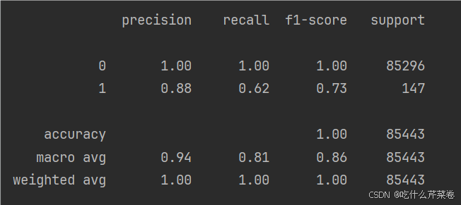
w_test_predicted = lr.predict(x_w_test)
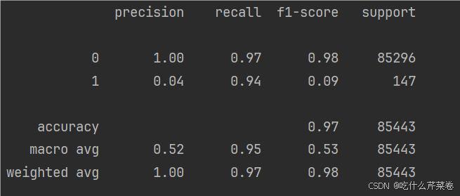
print(metrics.classification_report(y_w_test, w_test_predicted))

结果：

        显然，测试集的召回率大大提高，且更加平均，模型更加优秀

 

总结

        下采样方法适用于数据集中类别分布极不均衡的情况，能够平衡类别分布，可以减少过拟合的风险，使训练出的模型更加优秀。