Cross-Validation: Estimating Prediction Error

What is cross-validation?

Cross-Validation is a technique used in model selection to better estimate the test error of a predictive model. The idea behind cross-validation is to create a number of partitions of sample observations, known as the validation sets, from the training data set. After fitting a model on to the training data, its performance is measured against each validation set and then averaged, gaining a better assessment of how the model will perform when asked to predict for new observations. The number of partitions to construct depends on the number of observations in the sample data set as well as the decision made regarding the bias-variance trade-off, with more partitions leading to a smaller bias but a higher variance.

K-Fold cross-validation

This is the most common use of cross-validation. Observations are split into K partitions, the model is trained on K – 1 partitions, and the test error is predicted on the left out partition k. The process is repeated for k = 1,2…K and the result is averaged. If K=n, the process is referred to as Leave One Out Cross-Validation, or LOOCV for short. This approach has low bias, is computationally cheap, but the estimates of each fold are highly correlated. In this tutorial we will use K = 5.

Getting started

We will be using the boot package and data found in the MASSlibrary. Let’s see how cross-validation performs on the datasetcars, which measures the speed versus stopping distance of automobiles.

install.packages("boot")
require(boot)
library(MASS)
plot(speed~dist, data=cars, main = "Cars" ,
xlab = "Stopping Distance", ylab = "Speed")

Here is the plot:

Let’s apply a generalized linear model to our data, and see how our cross-validated error estimate changes with each degree polynomial.

glm.fit = glm(speed~dist, data=cars)
degree=1:5
cv.error5=rep(0,5)
for(d in degree){
glm.fit = glm(speed~poly(dist, d), data=cars)
cv.error5[d] = cv.glm(cars,glm.fit,K=5)$delta[1]
}

Here is the plot:

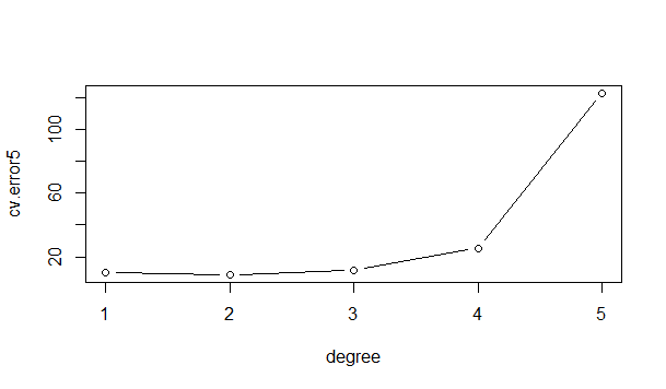
As you can see, a degree 1 or 2 polynomial seems to fit the model the closest while also holding the most predictive power. Since the difference is negligible, it is best to opt for the simpler model when possible. Notice how overfitting occurs after a certain degree polynomial, causing the model to lose its predictive performance.

Conclusion

Cross-validation is a good technique to test a model on its predictive performance. While a model may minimize the Mean Squared Error on the training data, it can be optimistic in its predictive error. The partitions used in cross-validation help to simulate an independent data set and get a better assessment of a model’s predictive performance.

Related Post

1. Interactive Performance Evaluation of Binary Classifiers
2. Predicting wine quality using Random Forests
3. Bayesian regression with STAN Part 2: Beyond normality
4. Hierarchical Clustering in R
5. Bayesian regression with STAN: Part 1 normal regression