A Hands-On Introduction to Time Series Classification (with Python Code)

Ref: https://medium.com/analytics-vidhya/a-hands-on-introduction-to-time-series-classification-with-python-code-48f8b442e7c1

Classifying time series data? Is that really possible? What could potentially be the use of doing that? These are just some of the questions you must have had when you read the title of this article. And it’s only fair — I had the exact same thoughts when I first came across this concept!

The time series data most of us are exposed to deals primarily with generating forecasts. Whether that’s predicting the demand or sales of a product, the count of passengers in an airline or the closing price of a particular stock, we are used to leveraging tried and tested time series techniques for forecasting requirements.

But as the amount of data being generated increases exponentially, so does the opportunity to experiment with new ideas and algorithms. Working with complex time series datasets is still a niche field, and it’s always helpful to expand your repertoire to include new ideas.

And that is what I aim to do in the article by introducing you to the novel concept of time series classification. We will first understand what this topic means and it’s applications in the industry. But we won’t stop at the theory part — we’ll get our hands dirty by working on a time series dataset and performing binary time series classification. Learning by doing — this will help you understand the concept in a practical manner as well.

If you have not worked on a time series problem before, I highly recommend first starting with some basic forecasting. You can go through the below article for starters:

A comprehensive beginner’s guide to create a Time Series Forecast (with Codes in Python)

Table of contents

1. Introduction to Time Series Classification
   1.1 ECG Signals
   1.2 Image Data
   1.3 Sensors
2. Setting up the Problem Statement
3. Reading and Understanding the Data
4. Preprocessing
5. Building our Time Series Classification Model

Introduction to Time Series Classification

Time series classification has actually been around for a while. But it has so far mostly been limited to research labs, rather than industry applications. But there is a lot of research going on, new datasets being created and a number of new algorithms being proposed. When I first came across this time series classification concept, my initial thought was — how can we classify a time series and what does a time series classification data look like? I’m sure you must be wondering the same thing.

As you can imagine, time series classification data differs from a regular classification problem since the attributes have an ordered sequence. Let’s have a look at some time series classification use cases to understand this difference.

1) Classifying ECG/EEG signals

ECG, or electrocardiogram, records the electrical activity of the heart and is widely be used to diagnose various heart problems. These ECG signals are captured using external electrodes.

For example, consider the following signal sample which represents the electrical activity for one heartbeat. The image on the left represents a normal heartbeat while the one adjacent to it represents a Myocardial Infarction.

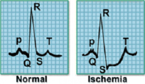
The data captured from the electrodes will be in time series form, and the signals can be classified into different classes. We can also classify EEG signals which record the electrical activity of the brain.

2) Image Classification

Images can also be in a sequential time-dependent format. Consider the following scenario:

Crops are grown in a particular field depending upon the weather conditions, soil fertility, availability of water and other external factors. A picture of this field is taken daily for 5 years and labeled with the name of the crop planted on the field. Do you see where I’m going with this? The images in the dataset are taken after a fixed time interval and have a defined sequence, which can be an important factor in classifying the images.

3) Classifying Motion Sensor Data

Sensors generate high-frequency data that can identify the movement of objects in their range. By setting up multiple wireless sensors and observing the change in signal strength in the sensors, we can identify the object’s direction of movement.

What other applications can you think of where we can apply time series classification? Let me know in the comments section below the article.

Setting up the Problem Statement

We will be working on the ‘Indoor User Movement Prediction‘ problem. In this challenge, multiple motion sensors are placed in different rooms and the goal is to identify whether an individual has moved across rooms, based on the frequency data captured from these motion sensors.

There are four motion sensors (A1, A2, A3, A4) placed across two rooms. Have a look at the below image which illustrates where the sensors are positioned in each room. The setup in these two rooms was created in 3 different pairs of rooms (group1, group2, group3).

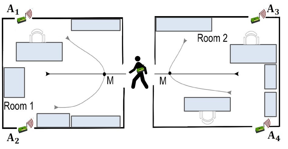
A person can move along any of the six pre-defined paths shown in the above image. If a person walks on path 2, 3, 4 or 6, he moves within the room. On the other hand, if a person follows path 1 or path 5, we can say that the person has moved between the rooms.

The sensor reading can be used to identify the position of a person at a given point in time. As the person moves in the room or across rooms, the reading in the sensor changes. This change can be used to identify the path of the person.

Now that the problem statement is clear, it’s time to get down to coding! In the next section, we will look at the dataset for the problem which should help clear up any lingering questions you might have on this statement. You can download the dataset from this link: Indoor User Movement Prediction.

Reading and Understanding the Data

Our dataset comprises of 316 files:

• 314 MovementAAL csv files containing the readings from motion sensors placed in the environment
• A Target csv file that contains the target variable for each MovementAAL file
• One Group Data csv file to identify which MovementAAL file belongs to which setup group
• The Path csv file that contains the path which the object took

Let’s have a look at the datasets. We’ll start by importing the necessary libraries.

import pandas as pd 
import numpy as np 
%matplotlib inline 
import matplotlib.pyplot as plt 
from os import listdir

from keras.preprocessing import sequence 
import tensorflow as tf 
from keras.models import Sequential 
from keras.layers import Dense 
from keras.layers import LSTM 
from keras.optimizers import Adam 
from keras.models import load_model 
from keras.callbacks import ModelCheckpoint

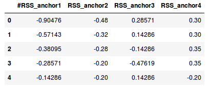
Before loading all the files, let’s take a quick sneak peek into the data we are going to deal with. Reading the first two files from the movement data:

df1 = pd.read_csv(‘/MovementAAL/dataset/MovementAAL_RSS_1.csv') df2 = pd.read_csv('/MovementAAL/dataset/MovementAAL_RSS_2.csv')

df1.head()

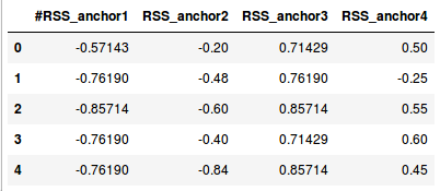
df2.head()

df1.shape, df2.shape

((27, 4), (26, 4))

The files contain normalized data from the four sensors — A1, A2, A3, A4. The length of the csv files (number of rows) vary, since the data corresponding to each csv is for a different duration. To simplify things, let us suppose the sensor data is collected every second. The first reading was for a duration of 27 seconds (so 27 rows), while another reading was for 26 seconds (so 26 rows).

We will have to deal with this varying length before we build our model. For now, we will read and store the values from the sensors in a list using the following code block:

path = 'MovementAAL/dataset/MovementAAL_RSS_'
sequences = list()
for i in range(1,315):
    file_path = path + str(i) + '.csv'
    print(file_path)
    df = pd.read_csv(file_path, header=0)
    values = df.values
    sequences.append(values)

targets = pd.read_csv('MovementAAL/dataset/MovementAAL_target.csv') 
targets = targets.values[:,1]

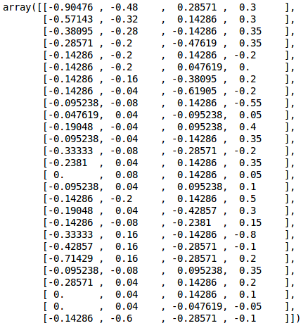
We now have a list ‘sequences’ that contains the data from the motion sensors and ‘targets’ which holds the labels for the csv files. When we print sequences[0], we get the values of sensors from the first csv file:

sequences[0]

As mentioned previously, the dataset was collected in three different pairs of rooms — hence three groups. This information can be used to divide the dataset into train, test and validation sets. We will load the DatasetGroup csv file now:

groups = pd.read_csv('MovementAAL/groups/MovementAAL_DatasetGroup.csv', header=0) 
groups = groups.values[:,1]

We will take the data from the first two sets for training purposes and the third group for testing.

Preprocessing Steps

Since the time series data is of varying length, we cannot directly build a model on this dataset. So how can we decide the ideal length of a series? There are multiple ways in which we can deal with it and here are a few ideas (I would love to hear your suggestions in the comment section):

• Pad the shorter sequences with zeros to make the length of all the series equal. In this case, we will be feeding incorrect data to the model
• Find the maximum length of the series and pad the sequence with the data in the last row
• Identify the minimum length of the series in the dataset and truncate all the other series to that length. However, this will result in a huge loss of data
• Take the mean of all the lengths, truncate the longer series, and pad the series which are shorter than the mean length

Let’s find out the minimum, maximum and mean length:

len_sequences = []
for one_seq in sequences:
    len_sequences.append(len(one_seq))
pd.Series(len_sequences).describe()

count    314.000000
mean      42.028662
std       16.185303
min       19.000000
25%       26.000000
50%       41.000000
75%       56.000000
max      129.000000
dtype: float64

Most of the files have lengths between 40 to 60. Just 3 files are coming up with a length more than 100. Thus, taking the minimum or maximum length does not make much sense. The 90th quartile comes out to be 60, which is taken as the length of sequence for the data. Let’s code it out:

#Padding the sequence with the values in last row to max length
to_pad = 129
new_seq = []
for one_seq in sequences:
    len_one_seq = len(one_seq)
    last_val = one_seq[-1]
    n = to_pad - len_one_seq
   
    to_concat = np.repeat(one_seq[-1], n).reshape(4, n).transpose()
    new_one_seq = np.concatenate([one_seq, to_concat])
    new_seq.append(new_one_seq)
final_seq = np.stack(new_seq)

#truncate the sequence to length 60
from keras.preprocessing import sequence
seq_len = 60
final_seq=sequence.pad_sequences(final_seq, maxlen=seq_len, padding='post', dtype='float', truncating='post')

Now that the dataset is prepared, we will separate it based on the groups. Preparing the train, validation and test sets:

train = [final_seq[i] for i in range(len(groups)) if (groups[i]==2)]
validation = [final_seq[i] for i in range(len(groups)) if groups[i]==1]
test = [final_seq[i] for i in range(len(groups)) if groups[i]==3]

train_target = [targets[i] for i in range(len(groups)) if (groups[i]==2)]
validation_target = [targets[i] for i in range(len(groups)) if groups[i]==1]
test_target = [targets[i] for i in range(len(groups)) if groups[i]==3]

train = np.array(train)
validation = np.array(validation)
test = np.array(test)

train_target = np.array(train_target)
train_target = (train_target+1)/2

validation_target = np.array(validation_target)
validation_target = (validation_target+1)/2

test_target = np.array(test_target)
test_target = (test_target+1)/2

Building a Time Series Classification model

We have prepared the data to be used for an LSTM (Long Short Term Memory) model. We dealt with the variable length sequence and created the train, validation and test sets. Let’s build a single layer LSTM network.

Note: You can get acquainted with LSTMs in this wonderfully explained tutorial. I would advice you to go through that first as it’ll help you understand how the below code works.

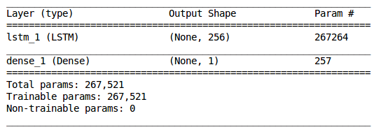
model = Sequential()
model.add(LSTM(256, input_shape=(seq_len, 4)))
model.add(Dense(1, activation='sigmoid'))

model.summary()

We will now train the model and monitor the validation accuracy:

adam = Adam(lr=0.001)
chk = ModelCheckpoint('best_model.pkl', monitor='val_acc', save_best_only=True, mode='max', verbose=1)
model.compile(loss='binary_crossentropy', optimizer=adam, metrics=['accuracy'])
model.fit(train, train_target, epochs=200, batch_size=128, callbacks=[chk], validation_data=(validation,validation_target))

#loading the model and checking accuracy on the test data
model = load_model('best_model.pkl')

from sklearn.metrics import accuracy_score
test_preds = model.predict_classes(test)
accuracy_score(test_target, test_preds)

I got an accuracy score of 0.78846153846153844. It’s quite a promising start but we can definitely improve the performance of the LSTM model by playing around with the hyperparameters, changing the learning rate, and/or the number of epochs as well.

End Notes

That brings us to the end of this tutorial. The idea behind penning this down was to introduce you to a whole new world in the time series spectrum in a practical manner.

Personally, I found the preprocessing step the most complex section of all the ones we covered. Yet, it is the most essential one as well (otherwise the whole point of time series data will fail!). Feeding the right data to the model is equally important when working on this kind of challenge.

Here is a really cool time series classification resource which I referred to and found the most helpful:

• Paper on “Predicting User Movements in Heterogeneous Indoor Environments by Reservoir Computing”

I would love to hear your thoughts and suggestions in the comment section below.

---

Originally published at www.analyticsvidhya.com on January 7, 2019.