


开始卷积之旅前先讲个游戏玩家的段子,当新闻中报道一些人工智能和比特币相关的内容时经常看到有人评论说“都是你们瞎搞,害得老子玩个魔兽显卡都换不起”。这个段子梗就在于下面我第一个介绍的部分GPU。正是由于AI热带来了对独立显卡的(特别是N卡)的爆炸式需求一下打破市场平衡,显卡价格水涨船高,才引起了游戏玩家门的吐槽。PS:要是早几年囤几箱N卡现在拿出来卖应该也可以换个房子了吧。。。
CPU和GPU的区别
简单理解是CPU是高级的可以做复杂逻辑运算的1个教授,GPU是低级的专注特定类型的一屋子小学生。
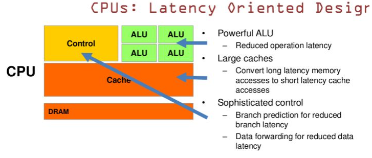

图中绿色代表计算单元,橙色代表存储单元,黄色代表控制单元,只从绿色所占的比例可以简单理解在处理单一低级任务时GPU要被CPU快很多,基本相差一个数量级。就像你要运算微积分傅里叶这玩意一个教授绝对秒杀一屋子小学生,但是如果计算十以内的加减法单位时间内一屋子小学生的运算量要秒杀一个教授。
Theano的使用
Theano可以理解为定义规则的基于python的编程语言,使用它主要有2个原因:
主要原因:可以使用GPU进行计算,效率比CPU计算高1个数量级。
次要原因:内置了很多黑科技,可以用简单的代码完成复杂的工作。
Theano的python包下载与安装,请参考《机器学习入门前准备》中的第二部分—扩展包下载和安装。
理论上需要搭建GPU环境的,但是我这可怜的A卡。。。说多了都是泪,越来越觉得搞人工智能还是个贵族工作。。。
默认大家都已经有一定编程基础了,直接上个样例代码配合实例解释下:
我这里要定义一个function,可以对x的平方求导:
import theano.tensor as T
from theano import function

#定义一个入参x
x = T.dscalar('x')
y = x**2
#grad函数,对公式y中的x求导
qy = T.grad(y,x)
#定义function,第一个参数是入参,集合形式;第二个参数是出参
f = function([x],qy)
qy = f(4)
print(qy)
#结果为8,其实就是求导
该注意的地方已经在注释中标明了,基本步骤就是定义变量、定义运算公式、将变量和运算公式组织成function、调用function这4个步骤。
直接再上个难度,用Theano来模拟单层网络的学习,通过BP方式训练一个与门:
import theano
import numpy as np
import theano.tensor as T
from theano import function
import random
#定义矩阵类型的入参x,训练集
x = T.matrix('x')
#因为w和b需要不断地学习,不断的被update,所以这里定义成shared
w = theano.shared(np.array([random.random(),random.random()]))
b = theano.shared(random.random())
#梯度步长
learning_rate = 0.1
z = T.dot(x,w)+b
#激活函数
a = 1/(1+T.exp(-z))
#定义第二个入参a_hat,训练集的目标值
a_hat = T.vector('a_hat')
#cost function使用的是交叉熵
cost = -(a_hat*T.log(a)+(1-a_hat)*T.log(1-a)).sum()
#对w和b分别求偏导
dw,db = T.grad(cost,[w,b])
#多了一个updates参数,该参数标识当function执行完毕后要更改shared类型的变量
#梯度下降
#w=w-learning_rate*dw
#b=b-learning_rate*db
train = function(
inputs = [x, a_hat],
outputs = [a, cost],
updates = [[w,w-learning_rate*dw],[b,b-learning_rate*db]]
)
#训练集
inputs = [[0,0],[0,1],[1,0],[1,1]]
outputs = [0,0,0,1]
costResult = []
for iteration in range(3000):
pred, cost_iter = train(inputs,outputs)
costResult.append(cost_iter)
for i in range(len(inputs)):
print('The output for x1=%d | x2=%d is %.2f' % (inputs[i][0],inputs[i][1],pred[i])
)
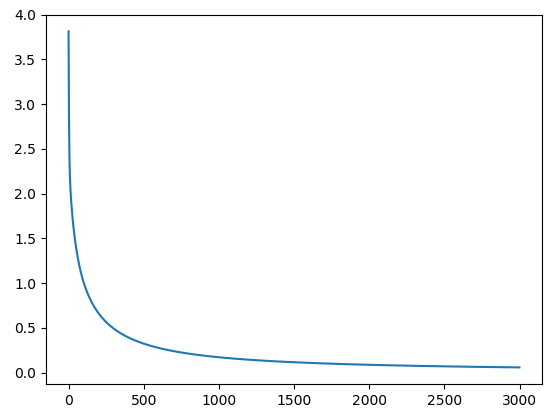
#图形化观察cost function的速度
import matplotlib.pyplot as plt
plt.plot(costResult)
plt.show()输出结果打印:
The output for x1=0 | x2=0 is 0.00
The output for x1=0 | x2=1 is 0.02
The output for x1=1 | x2=0 is 0.02
The output for x1=1 | x2=1 is 0.98
Cost function训练效率:
OK,理解下来有点难度了,下面是个更高难度的,我们用theano来实现含有一个隐藏层的网络来进行mnist手写数字识别的训练。
隐藏层用全连接,全连接的概念后面有详细说明:
#最原始的,直接全连接网络
class FullyConnectedLayer(object):

    def __init__(self, n_in, n_out, activation_fn=sigmoid, p_dropout=0.0):
        self.n_in = n_in
        self.n_out = n_out
        #设计激活函数
        self.activation_fn = activation_fn
        self.p_dropout = p_dropout
        # 权重初始化采用了标准化
        self.w = theano.shared(
            np.asarray(
                np.random.normal(
                    loc=0.0, scale=np.sqrt(1.0/n_out), size=(n_in, n_out)),
                dtype=theano.config.floatX),
            name='w', borrow=True)
        self.b = theano.shared(
            np.asarray(np.random.normal(loc=0.0, scale=1.0, size=(n_out,)),
                       dtype=theano.config.floatX),
            name='b', borrow=True)
        self.params = [self.w, self.b]

    #参与准确率计算的,只有y_out,但是传递到后面网络的是output_dropout
    def set_inpt(self, inpt, inpt_dropout, mini_batch_size):
        self.inpt = inpt.reshape((mini_batch_size, self.n_in))
        self.output = self.activation_fn(
            (1-self.p_dropout)*T.dot(self.inpt, self.w) + self.b)
        self.y_out = T.argmax(self.output, axis=1)
        self.inpt_dropout = dropout_layer(
            inpt_dropout.reshape((mini_batch_size, self.n_in)), self.p_dropout)
        self.output_dropout = self.activation_fn(
            T.dot(self.inpt_dropout, self.w) + self.b)

    def accuracy(self, y):
        "Return the accuracy for the mini-batch."
        return T.mean(T.eq(y, self.y_out))
输出层用柔性最大:
#柔性最大层
class SoftmaxLayer(object):

    def __init__(self, n_in, n_out, p_dropout=0.0):
        self.n_in = n_in
        self.n_out = n_out
        self.p_dropout = p_dropout
        self.w = theano.shared(
            np.zeros((n_in, n_out), dtype=theano.config.floatX),
            name='w', borrow=True)
        self.b = theano.shared(
            np.zeros((n_out,), dtype=theano.config.floatX),
            name='b', borrow=True)
        self.params = [self.w, self.b]

    def set_inpt(self, inpt, inpt_dropout, mini_batch_size):
        self.inpt = inpt.reshape((mini_batch_size, self.n_in))
        #柔性最大算法获得结果
        self.output = softmax((1-self.p_dropout)*T.dot(self.inpt, self.w) + self.b)
        self.y_out = T.argmax(self.output, axis=1)
        self.inpt_dropout = dropout_layer(
            inpt_dropout.reshape((mini_batch_size, self.n_in)), self.p_dropout)
        self.output_dropout = softmax(T.dot(self.inpt_dropout, self.w) + self.b)

    #cost function使用对数似然
    def cost(self, net):
        "Return the log-likelihood cost."
        return -T.mean(T.log(self.output_dropout)[T.arange(net.y.shape[0]), net.y])

    def accuracy(self, y):
        "Return the accuracy for the mini-batch."
        return T.mean(T.eq(y, self.y_out))
整个网络构建如下:
class Network(object):
    def __init__(self, layers, mini_batch_size):
        self.layers = layers
        self.mini_batch_size = mini_batch_size
        #params是高维的layer的参数
        self.params = [param for layer in self.layers for param in layer.params]
        #theano定义输入输出
        self.x = T.matrix("x")
        self.y = T.ivector("y")
        #确定第一层
        init_layer = self.layers[0]
        #初始化输入层
        init_layer.set_inpt(self.x, self.x, self.mini_batch_size)
        #初始化第一层后面的所有层
        #所谓的初始化就是给每层指定输入输出
        for j in range(1, len(self.layers)):
            prev_layer, layer  = self.layers[j-1], self.layers[j]
            layer.set_inpt(prev_layer.output, prev_layer.output_dropout, self.mini_batch_size)
        self.output = self.layers[-1].output
        self.output_dropout = self.layers[-1].output_dropout

    def SGD(self, training_data, epochs, mini_batch_size, eta,
            validation_data, test_data, lmbda=0.0):
        training_x, training_y = training_data
        validation_x, validation_y = validation_data
        test_x, test_y = test_data

        #计算拆成了多少片段
        num_training_batches = int(size(training_data)/mini_batch_size)
        num_validation_batches = int(size(validation_data)/mini_batch_size)
        num_test_batches = int(size(test_data)/mini_batch_size)


        l2_norm_squared = sum([(layer.w**2).sum() for layer in self.layers])
        #这里不清楚为什么cost是这个公式?
        cost = self.layers[-1].cost(self)+0.5*lmbda*l2_norm_squared/num_training_batches
        grads = T.grad(cost, self.params)
        #梯度下降
        updates = [(param, param-eta*grad)
                   for param, grad in zip(self.params, grads)]

        #定义一个变量i,i代表的是第几波次mini_batch
        i = T.lscalar()
        #梯度下降学习的function
        train_mb = theano.function(
            [i], cost, updates=updates,
            givens={
                self.x:
                training_x[i*self.mini_batch_size: (i+1)*self.mini_batch_size],
                self.y:
                training_y[i*self.mini_batch_size: (i+1)*self.mini_batch_size]
            })
        #求validate的准确率的function
        validate_mb_accuracy = theano.function(
            [i], self.layers[-1].accuracy(self.y),
            givens={
                self.x:
                validation_x[i*self.mini_batch_size: (i+1)*self.mini_batch_size],
                self.y:
                validation_y[i*self.mini_batch_size: (i+1)*self.mini_batch_size]
            })
        # 求test的准确率的function
        test_mb_accuracy = theano.function(
            [i], self.layers[-1].accuracy(self.y),
            givens={
                self.x:
                test_x[i*self.mini_batch_size: (i+1)*self.mini_batch_size],
                self.y:
                test_y[i*self.mini_batch_size: (i+1)*self.mini_batch_size]
            })
        #求第i组mini_batch预测结果的function
        self.test_mb_predictions = theano.function(
            [i], self.layers[-1].y_out,
            givens={
                self.x:
                test_x[i*self.mini_batch_size: (i+1)*self.mini_batch_size]
            })
        # Do the actual training
        best_validation_accuracy = 0.0
        for epoch in range(epochs):
            #对每一小块进行训练,minibatch_index是分段的序号
            #训练num_training_batches次,每次训练mini_batch_size个
            for minibatch_index in range(num_training_batches):
                #iteration是每条训练数据的序号了
                iteration = num_training_batches*epoch+minibatch_index
                #训练1000条记录后打印一行,没实际意义
                if iteration % 1000 == 0:
                    print("Training mini-batch number {0}".format(iteration))
                #训练一段并完成该段的bp,返回的是cost function函数结果
                cost_ij = train_mb(minibatch_index)
                #下面这行代码的意思是:当本次内循环全部执行完,也就是说训练了,需要做一次总结
                if (iteration+1) % num_training_batches == 0:
                    validation_accuracy = np.mean(
                        [validate_mb_accuracy(j) for j in range(num_validation_batches)])
                    print("Epoch {0}: validation accuracy {1:.2%}".format(
                        epoch, validation_accuracy))
                    #有可能过拟合,所以这里维护下中间最优的信息
                    if validation_accuracy >= best_validation_accuracy:
                        print("This is the best validation accuracy to date.")
                        best_validation_accuracy = validation_accuracy
                        best_iteration = iteration
                        if test_data:
                            test_accuracy = np.mean(
                                [test_mb_accuracy(j) for j in range(num_test_batches)])
                            print('The corresponding test accuracy is {0:.2%}'.format(
                                test_accuracy))
        print("Finished training network.")
        print("Best validation accuracy of {0:.2%} obtained at iteration {1}".format(
            best_validation_accuracy, best_iteration))
        print("Corresponding test accuracy of {0:.2%}".format(test_accuracy))
相关的模块导入、方法定义、以及输入层数据加载:
import numpy as np
import theano
import theano.tensor as T
from theano.tensor.nnet import conv
from theano.tensor.nnet import softmax
from theano.tensor import shared_randomstreams
import pickle
import gzip

def linear(z): return z
def ReLU(z): return T.maximum(0.0, z)
from theano.tensor.nnet import sigmoid
from theano.tensor import tanh
from theano.tensor.signal import pool

def load_data_shared(filename="C:\\2018\\DNN\\mnist.pkl.gz"):
    f = gzip.open(filename, 'rb')
    training_data, validation_data, test_data = pickle.load(f,encoding='bytes')
    f.close()
    def shared(data):
        shared_x = theano.shared(
            np.asarray(data[0], dtype=theano.config.floatX), borrow=True)
        shared_y = theano.shared(
            np.asarray(data[1], dtype=theano.config.floatX), borrow=True)
        return shared_x, T.cast(shared_y, "int32")
    return [shared(training_data), shared(validation_data), shared(test_data)]
有了这些原材料,只需要构造network对象然后调用其SGD方法就可以训练我们的网络了:
net = Network([FullyConnectedLayer(n_in=784, n_out=100),SoftmaxLayer(n_in=100, n_out=10)],mini_batch_size)
net.SGD(training_data,60,mini_batch_size,0.1,validation_data,test_data)
这里只有一个隐藏层,在《消失的梯度问题(vanishinggradient problem)》中我们介绍过随着网络层次的加深会引起梯度的不稳定,为了解决这个问题,我们下面要引入卷积网络CNN的概念。
首先,与卷积相对的是全连接,网络中的神经元与相邻层上的每个神经元都建立连接,如图:
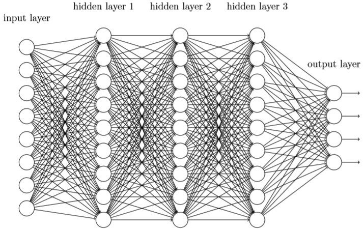
全连接网络在处理图像时讲每个像素看成独立的输入点,忽略了它们的位置关系,这样将带来一个问题,相同的敏感信息当初现在图像的不同位置时分析的结果是有差别的。机器学习中的《k-近邻算法及代码》一样存在着类似的问题。所以引入卷积神经网络的概念,将输入看成28*28像素的平面,不再是前面的1*748的纵向的列。
卷积神经网络的核心有3个概念:局部感受视野、共享权重和偏置、池化pooling。
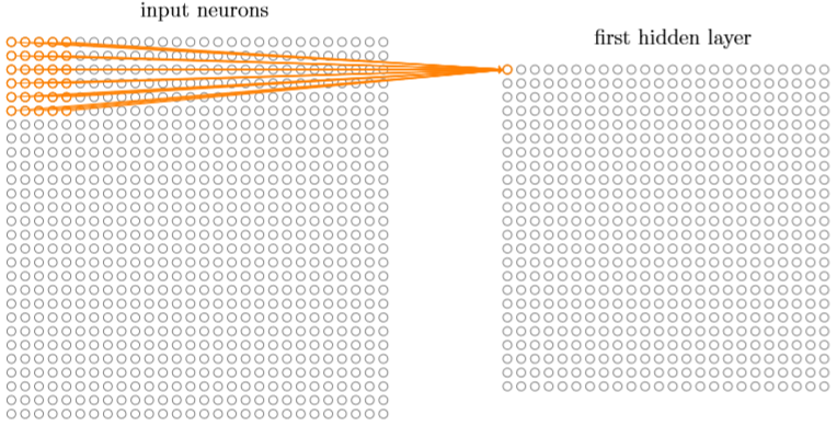
局部感受视野:
我们将输入图像进行小的、局部区域的连接,也就是说隐藏层中的每个神经元会连接到输入神经元的一小个区域,如下图就是一个5*5的局部感受视野对应于25个输入像素,该5*5的局部感受视野每个像素点使用一个权重w,然后公用一个偏置b,共26个变量。
然后局部感受视野依次按照跨度连续的平移,例如如果跨度是1,向右平移一次,如下图:
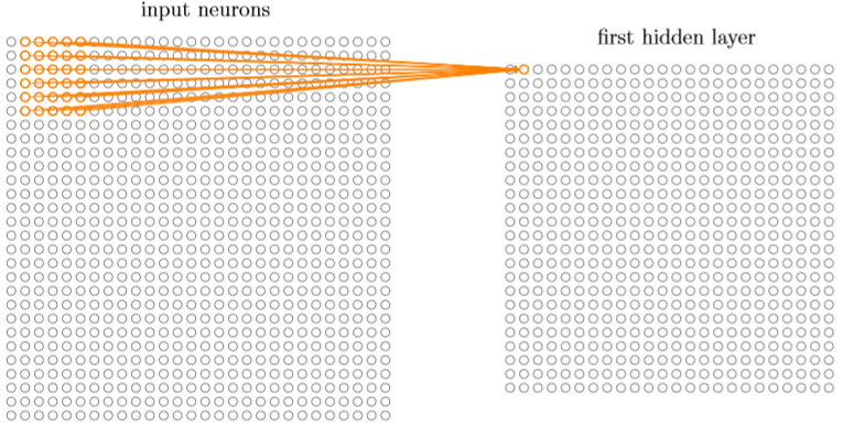
如此重复构建起第一个隐藏层,如果28*28的输入网络,按照跨度为1局部视野为5*5,最终将形成一个28-5+1的方阵网络
共享权重和偏置:
以上所有局部感受视野的25个权重加1个偏置都是公用的,这是卷积网络保持图像平移不变性的核心算法。例如下图中的两只猫,在共享权重和偏置的基础上2张图片求得的w和b应该是一样的。
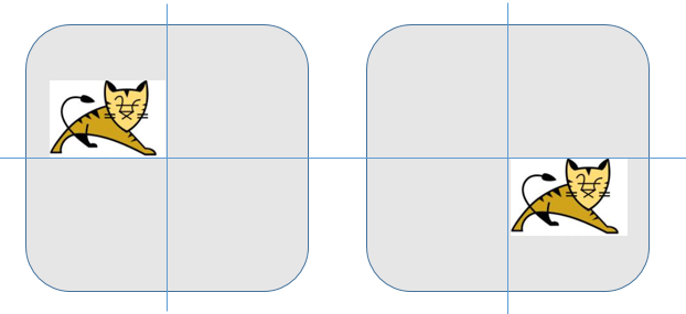
一组共享权重和偏置又被称为一个卷积核或滤波器,它所干的事情更像是扫描图片发现特征信息,唯一不同的是被扫描到的特征信息可能出现在图片的不同位置罢了。
池化pooling:
池化是对卷积后的数据做进一步浓缩的过程,例如下图是利用2*2的像素对上面24*24的卷积产出做池化:
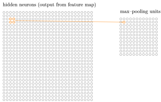
与卷积层不同的是,第一:池化是成比例的浓缩,而不是卷积跨度的平移,例如24*24的网络被2*2的池化浓缩,产出是12*12的网络。第二:池化的过程不存在权重和偏置的概念,一般是取像素中最大,又或者平方和的平方根,再或者取均值做为池化产出像素点的值,分别称为Max-pooling、L2-pooling和mean-pooling,无论哪种池化技术,本质的意义都是为了浓缩,减少后面网络处理时的压力。
下面我们利用卷积网络+全连接网络来重新搭建一个手写数字识别的学习网络:
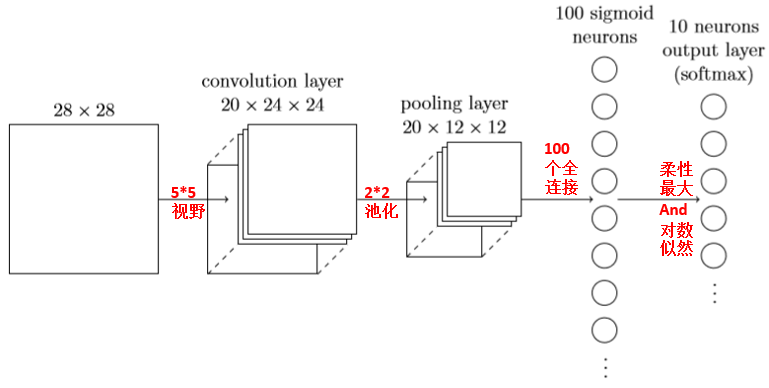
PS:有人将卷积层和池化层分开看成两个隐藏层,也有人认为一次卷积+一次池化属于一个隐藏层,但无论如何我们这里的网络有2个或者2个以上的隐藏层了,所以可以称之为深度学习了。
代码增加一个卷积层:
#卷积层
class ConvPoolLayer(object):
    def __init__(self, filter_shape, image_shape, poolsize=(2, 2),
                 activation_fn=sigmoid):
        #卷积层(节点数、输入特性数、高、宽)
        self.filter_shape = filter_shape
        #图片输入(mini_batch_size,输入特性数、高、宽)
        self.image_shape = image_shape
        #pool层(高、宽)
        self.poolsize = poolsize
        #激活函数
        self.activation_fn=activation_fn
        #这里n_out的处理很有意思,规范化初始化权重
        n_out = (filter_shape[0]*np.prod(filter_shape[2:])/np.prod(poolsize))
        self.w = theano.shared(
            np.asarray(
                np.random.normal(loc=0, scale=np.sqrt(1.0/n_out), size=filter_shape),
                dtype=theano.config.floatX),
            borrow=True)
        self.b = theano.shared(
            np.asarray(
                np.random.normal(loc=0, scale=1.0, size=(filter_shape[0],)),
                dtype=theano.config.floatX),
            borrow=True)
        self.params = [self.w, self.b]

    def set_inpt(self, inpt, inpt_dropout, mini_batch_size):
        self.inpt = inpt.reshape(self.image_shape)
        #求卷积的函数
        conv_out = conv.conv2d(
            input=self.inpt, filters=self.w, filter_shape=self.filter_shape,
            image_shape=self.image_shape)
        #pooling
        pooled_out = pool.pool_2d(
            input=conv_out, ds=self.poolsize, ignore_border=True)
        self.output = self.activation_fn(
            pooled_out + self.b.dimshuffle('x', 0, 'x', 'x'))
        #卷积没有弃权
        self.output_dropout = self.output
新网络架构如下:
net = Network([ConvPoolLayer(image_shape=(mini_batch_size,1,28,28),
                             filter_shape=(20,1,5,5),
                             poolsize=(2,2),activation_fn=ReLU),
               FullyConnectedLayer(n_in=20*12*12, n_out=100,activation_fn=ReLU),
               SoftmaxLayer(n_in=100, n_out=10)],mini_batch_size)
net.SGD(training_data,60,mini_batch_size,0.05,validation_data,test_data,lmbda=0.1)
#弃权,隐藏部分节点变成新的网络
def dropout_layer(layer, p_dropout):
    srng = shared_randomstreams.RandomStreams(
        np.random.RandomState(0).randint(999999))
    mask = srng.binomial(n=1, p=1-p_dropout, size=layer.shape)
    return layer*T.cast(mask, theano.config.floatX)
最后看个香港中文大学Sun Yi开发出的人脸识别的卷积网络,能达到99.15%的准确率,请注意它的全连接层对接着两个卷积层,使其可以学习到局部和全局的特性。
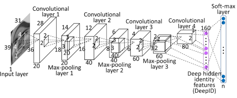
这里给出这个案例是为了说明对于深度学习很多时候我们对于其原理并没有足够的把握去推论或证明,我们可以通过大量的试验和创新式的设计去不断的尝试出更好表现的神经网络。


 2045
2045


 被折叠的 条评论
为什么被折叠?
被折叠的 条评论
为什么被折叠?
 到【灌水乐园】发言


