深度学习笔记一：稀疏自编码器

最新推荐文章于 2023-01-08 09:47:07 发布

CH-Yuan

最新推荐文章于 2023-01-08 09:47:07 发布

阅读量3.4k

点赞数

分类专栏：机器学习

本文链接：https://blog.csdn.net/yuanchheneducn/article/details/46453059

版权

机器学习专栏收录该内容

26 篇文章 0 订阅

订阅专栏

开始学习深度学习了，既然确定目标就要努力前行！为自己加油！——2015.6.11

Sparse Encoder

1.神经网络
概念：假设我们有训练样本集 (x(^ i),y(^ i)) ，那么神经网络算法能够提供一种复杂且非线性的假设模型 h_{W,b}(x) ，它具有参数 W, b ，可以以此参数来拟合我们的数据。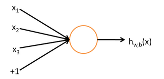这里写图片描述
激活函数：
f(z)=sigmoid(z)=1/(1+exp(-z))
导数：f’(z)=f(z)(1-f(z)) 很重要，求代价函数极值的时候要用到
模型：
一个简单的神经网络，只有输入层，一个隐藏层和输出层组成。每加一层就相当于对输入多进行一次非线性处理，进而形成复杂的目标函数hw,b(x).
(https://img-blog.csdn.net/20150611084555088)
目标值从前往后计算：
Z2=W1*data+b1
a2=f(Z2)
Z3=W2*a2+b2
a3=f(Z3)
目标函数的代价函数：
第一部分是：直接误差——m个输入的平均误差
第二部分是：权值惩罚——所有W元素的平方和，目的是为了减少权重的幅度，防止过度拟合
(https://img-blog.csdn.net/20150611085816673)
为使代价函数最小，可以使用批梯度下降法，从而确定参数W1，W2，b1,b2。
步骤：（1）给W1,W2,b1,b2初始值：初始值设计很关键，否则将会得到不好的结果，练习里面是这样设计的：

r  = sqrt(6) / sqrt(hiddenSize+visibleSize+1);   % we'll choose weights uniformly from the interval [-r, r]
W1 = rand(hiddenSize, visibleSize) * 2 * r - r;
W2 = rand(visibleSize, hiddenSize) * 2 * r - r;

b1 = zeros(hiddenSize, 1);
b2 = zeros(visibleSize, 1);

（2）需要给出代价函数:即上述代码公式
（3）需要给出代价函数对W和b的偏导
这里写图片描述
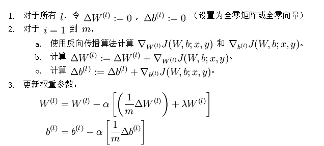
说明：这里需要的是后面有的1/m括号里的部分。括号里的第一部分其实就是每个输入对W,b求导值的平均。
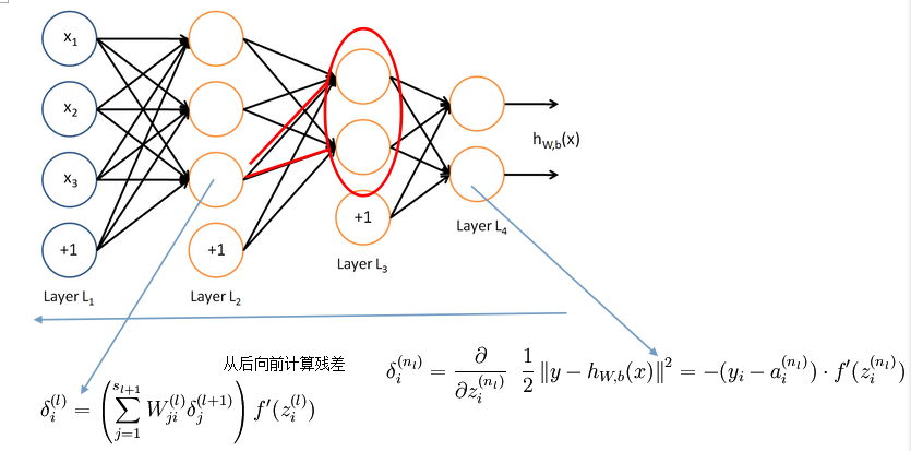
2、反向传导
这部分很关键，用于计算每个输入对的求导。为了对W求导，先对Z求导，对Z求导的结果就是残差。从后向前计算，有点类似于计算图的关键路径的计算方法。
这里写图片描述

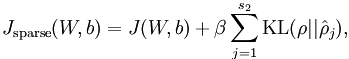
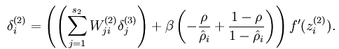
3、稀疏自编码器
代价函数和W偏导与普通神经网络有一点区别，代价函数需要加入稀疏代价。
这里写图片描述

这里写图片描述

心得：感觉稀疏自编码器就是对输入进行压缩表示，前面编码，最后一层解码。做个实验试了一下两个隐藏层的情况，想第一次发现边，第二次发现拐角，然而效果好差！翻了一下教程，发现后面有专门的栈式自编码器，汗~~~不过至少说明自己思考的方向是对滴~

代码完成中出现的问题：
错误总结：

Jcost=(0.5/m)*sum(sum((a3-data).^2));   
%%正确sum((a3-data).^2)，写成sum(a3-data).^2导致错误，找了好久的原因啊，原来是因为一对括号！

Jweight=0.5*(sum(sum(W1.^2))+sum(sum(W2.^2)));
%%写成了Jweight=0.5*sum(sum(W1.^2))+sum(sum(W2.^2));还是少了括号!!

经验：
minFun的用法

addpath minFunc/
options.Method = 'lbfgs'; % Here, we use L-BFGS to optimize our cost
                          % function. Generally, for minFunc to work, you
                          % need a function pointer with two outputs: the
                          % function value and the gradient. In our problem,
                          % sparseAutoencoderCost.m satisfies this.
options.maxIter = 400;    % Maximum number of iterations of L-BFGS to run 
options.display = 'on';


[opttheta, cost] = minFunc( @(p) sparseAutoencoderCost(p, ...
                                   visibleSize, hiddenSize, ...
                                   lambda, sparsityParam, ...
                                   beta, patches), ...
                              theta, options);
                              %需要提供一个返回代价函数和偏导的函数sparseAutoencoderCost

sparseAutoencoderCost.h

function [cost,grad] = sparseAutoencoderCost(theta, visibleSize, hiddenSize, ...
                                             lambda, sparsityParam, beta, data)

% visibleSize: the number of input units (probably 64) 
% hiddenSize: the number of hidden units (probably 25) 
% lambda: weight decay parameter
% sparsityParam: The desired average activation for the hidden units (denoted in the lecture
%                           notes by the greek alphabet rho, which looks like a lower-case "p").
% beta: weight of sparsity penalty term
% data: Our 64x10000 matrix containing the training data.  So, data(:,i) is the i-th training example. 

% The input theta is a vector (because minFunc expects the parameters to be a vector). 
% We first convert theta to the (W1, W2, b1, b2) matrix/vector format, so that this 
% follows the notation convention of the lecture notes. 

W1 = reshape(theta(1:hiddenSize*visibleSize), hiddenSize, visibleSize);
W2 = reshape(theta(hiddenSize*visibleSize+1:2*hiddenSize*visibleSize), visibleSize, hiddenSize);
b1 = theta(2*hiddenSize*visibleSize+1:2*hiddenSize*visibleSize+hiddenSize);
b2 = theta(2*hiddenSize*visibleSize+hiddenSize+1:end);

% Cost and gradient variables (your code needs to compute these values). 
% Here, we initialize them to zeros. 
cost = 0;
W1grad = zeros(size(W1)); 
W2grad = zeros(size(W2));
b1grad = zeros(size(b1)); 
b2grad = zeros(size(b2));

%% ---------- YOUR CODE HERE --------------------------------------
%  Instructions: Compute the cost/optimization objective J_sparse(W,b) for the Sparse Autoencoder,
%                and the corresponding gradients W1grad, W2grad, b1grad, b2grad.
%
% W1grad, W2grad, b1grad and b2grad should be computed using backpropagation.
% Note that W1grad has the same dimensions as W1, b1grad has the same dimensions
% as b1, etc.  Your code should set W1grad to be the partial derivative of J_sparse(W,b) with
% respect to W1.  I.e., W1grad(i,j) should be the partial derivative of J_sparse(W,b) 
% with respect to the input parameter W1(i,j).  Thus, W1grad should be equal to the term 
% [(1/m) \Delta W^{(1)} + \lambda W^{(1)}] in the last block of pseudo-code in Section 2.2 
% of the lecture notes (and similarly for W2grad, b1grad, b2grad).
% 
% Stated differently, if we were using batch gradient descent to optimize the parameters,
% the gradient descent update to W1 would be W1 := W1 - alpha * W1grad, and similarly for W2, b1, b2. 
% 
%%%%%%%%%%%%%%%%%%%%
%%%%%%%%%%%%%%%%%%%%ych代码
Jcost = 0;%直接误差
Jweight = 0;%权值惩罚
Jsparse = 0;%稀疏性惩罚
[n m] = size(data);%m为样本的个数，n为样本的特征数
% 
% %前向算法计算各神经网络节点的线性组合值和active值
z2=W1*data+repmat(b1,1,m);
a2=sigmoid(z2);
z3=W2*a2+repmat(b2,1,m);
a3=sigmoid(z3);


 Jcost=(0.5/m)*sum(sum((a3-data).^2));   %%正确sum((a3-data).^2)，写成sum(a3-data).^2导致错误，找了好久的原因啊，原来是因为一对括号！
 Jweight=0.5*(sum(sum(W1.^2))+sum(sum(W2.^2)));
rho=(1/m).*sum(a2,2);
Jsparse=sum(sparsityParam.*log(sparsityParam./rho)+(1-sparsityParam).*log((1-sparsityParam)./(1-rho)));

cost=Jcost+lambda*Jweight+beta*Jsparse;


d3=-(data-a3).*(sigmoid(z3).*(1-sigmoid(z3)));
sterm = beta*(-sparsityParam./rho+(1-sparsityParam)./(1-rho));
d2=(W2'*d3+repmat(sterm,1,m)).*(sigmoid(z2).*(1-sigmoid(z2)));


W1grad=(1/m).*(d2*data')+lambda.*W1;
W2grad=(1/m).*(d3*a2')+lambda.*W2;
b1grad=(1/m).*sum(d2,2);
b2grad=(1/m).*sum(d3,2);
%-------------------------------------------------------------------
% After computing the cost and gradient, we will convert the gradients back
% to a vector format (suitable for minFunc).  Specifically, we will unroll
% your gradient matrices into a vector.

grad = [W1grad(:) ; W2grad(:) ; b1grad(:) ; b2grad(:)];

end

function sigm = sigmoid(x)

    sigm = 1 ./ (1 + exp(-x));
end