改善深层神经网络：超参数调试、正则化以及优化 第一周作业2

Regularization

Welcome to the second assignment of this week. Deep Learning models have so much flexibility and capacity that overfitting can be a serious problem, if the training dataset is not big enough. Sure it does well on the training set, but the learned network doesn’t generalize to new examples that it has never seen!

You will learn to: Use regularization in your deep learning models.

Let’s first import the packages you are going to use.

输入：

import numpy as np
import matplotlib.pyplot as plt
from reg_utils import sigmoid, relu, plot_decision_boundary, initialize_parameters, load_2D_dataset, predict_dec
from reg_utils import compute_cost, predict, forward_propagation, backward_propagation, update_parameters
import sklearn
import sklearn.datasets
import scipy.io

plt.rcParams['figure.figsize'] = (7.0, 4.0) # set default size of plots
plt.rcParams['image.interpolation'] = 'nearest'
plt.rcParams['image.cmap'] = 'gray'

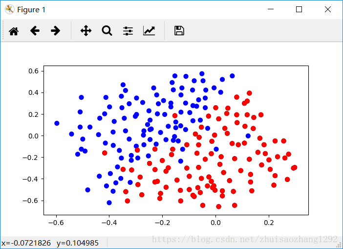
train_X, train_Y, test_X, test_Y = load_2D_dataset()

 

输出：

 

1 - Non-regularized model

You will use the following neural network (already implemented for you below). This model can be used: 
- in regularization mode – by setting the lambd input to a non-zero value. We use “lambd” instead of “lambda” because “lambda” is a reserved keyword in Python.

- in dropout mode – by setting the keep_prob to a value less than one

You will first try the model without any regularization. Then, you will implement: 
- L2 regularization – functions: “compute_cost_with_regularization()” and “backward_propagation_with_regularization()” 
- Dropout – functions: “forward_propagation_with_dropout()” and “backward_propagation_with_dropout()”

In each part, you will run this model with the correct inputs so that it calls the functions you’ve implemented. Take a look at the code below to familiarize yourself with the model.

 

Let’s train the model without any regularization, and observe the accuracy on the train/test sets.

输入：

import numpy as np
import matplotlib.pyplot as plt
from reg_utils import sigmoid, relu, plot_decision_boundary, initialize_parameters, load_2D_dataset, predict_dec
from reg_utils import compute_cost, predict, forward_propagation, backward_propagation, update_parameters
import sklearn
import sklearn.datasets
import scipy.io

def compute_cost_with_regularization(A3, Y, parameters, lambd):
    """
    Implement the cost function with L2 regularization. See formula (2) above.

    Arguments:
    A3 -- post-activation, output of forward propagation, of shape (output size, number of examples)
    Y -- "true" labels vector, of shape (output size, number of examples)
    parameters -- python dictionary containing parameters of the model

    Returns:
    cost - value of the regularized loss function (formula (2))
    """
    m = Y.shape[1]
    W1 = parameters["W1"]
    W2 = parameters["W2"]
    W3 = parameters["W3"]

    cross_entropy_cost = compute_cost(A3, Y) # This gives you the cross-entropy part of the cost

    ### START CODE HERE ### (approx. 1 line)
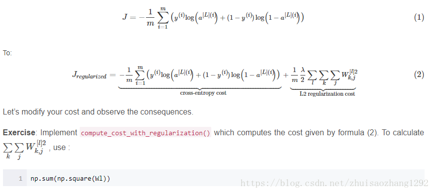
    L2_regularization_cost =(1./m)*(lambd/2)*(np.sum(np.square(W1)) + np.sum(np.square(W2)) + np.sum(np.square(W3)))
    ### END CODER HERE ###

    cost = cross_entropy_cost + L2_regularization_cost

    return cost

def backward_propagation_with_regularization(X, Y, cache, lambd):
    """
    Implements the backward propagation of our baseline model to which we added an L2 regularization.

    Arguments:
    X -- input dataset, of shape (input size, number of examples)
    Y -- "true" labels vector, of shape (output size, number of examples)
    cache -- cache output from forward_propagation()
    lambd -- regularization hyperparameter, scalar

    Returns:
    gradients -- A dictionary with the gradients with respect to each parameter, activation and pre-activation variables
    """

    m = X.shape[1]
    (Z1, A1, W1, b1, Z2, A2, W2, b2, Z3, A3, W3, b3) = cache

    dZ3 = A3 - Y

    ### START CODE HERE ### (approx. 1 line)
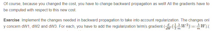
    dW3 = 1./m * np.dot(dZ3, A2.T) + (lambd/m)*W3
    ### END CODE HERE ###
    db3 = 1./m * np.sum(dZ3, axis=1, keepdims = True)

    dA2 = np.dot(W3.T, dZ3)
    dZ2 = np.multiply(dA2, np.int64(A2 > 0))
    ### START CODE HERE ### (approx. 1 line)
    dW2 = 1./m * np.dot(dZ2, A1.T) + (lambd/m)*W2
    ### END CODE HERE ###
    db2 = 1./m * np.sum(dZ2, axis=1, keepdims = True)

    dA1 = np.dot(W2.T, dZ2)
    dZ1 = np.multiply(dA1, np.int64(A1 > 0))
    ### START CODE HERE ### (approx. 1 line)
    dW1 = 1./m * np.dot(dZ1, X.T) + (lambd/m)*W1
    ### END CODE HERE ###
    db1 = 1./m * np.sum(dZ1, axis=1, keepdims = True)

    gradients = {"dZ3": dZ3, "dW3": dW3, "db3": db3,"dA2": dA2,
                 "dZ2": dZ2, "dW2": dW2, "db2": db2, "dA1": dA1, 
                 "dZ1": dZ1, "dW1": dW1, "db1": db1}

    return gradients

def forward_propagation_with_dropout(X, parameters, keep_prob = 0.5):
    """
    Implements the forward propagation: LINEAR -> RELU + DROPOUT -> LINEAR -> RELU + DROPOUT -> LINEAR -> SIGMOID.

    Arguments:
    X -- input dataset, of shape (2, number of examples)
    parameters -- python dictionary containing your parameters "W1", "b1", "W2", "b2", "W3", "b3":
                    W1 -- weight matrix of shape (20, 2)
                    b1 -- bias vector of shape (20, 1)
                    W2 -- weight matrix of shape (3, 20)
                    b2 -- bias vector of shape (3, 1)
                    W3 -- weight matrix of shape (1, 3)
                    b3 -- bias vector of shape (1, 1)
    keep_prob - probability of keeping a neuron active during drop-out, scalar

    Returns:
    A3 -- last activation value, output of the forward propagation, of shape (1,1)
    cache -- tuple, information stored for computing the backward propagation
    """

    np.random.seed(1)

    # retrieve parameters
    W1 = parameters["W1"]
    b1 = parameters["b1"]
    W2 = parameters["W2"]
    b2 = parameters["b2"]
    W3 = parameters["W3"]
    b3 = parameters["b3"]

    # LINEAR -> RELU -> LINEAR -> RELU -> LINEAR -> SIGMOID
    Z1 = np.dot(W1, X) + b1
    A1 = relu(Z1)
    ### START CODE HERE ### (approx. 4 lines)         # Steps 1-4 below correspond to the Steps 1-4 described above. 
    D1 = np.random.rand(A1.shape[0],A1.shape[1])      # Step 1: initialize matrix D1 = np.random.rand(..., ...)
    D1 = np.where(D1 <= keep_prob, 1, 0)              # Step 2: convert entries of D1 to 0 or 1 (using keep_prob as the threshold)
    A1 = A1 * D1                                      # Step 3: shut down some neurons of A1
    A1 = A1 / keep_prob                               # Step 4: scale the value of neurons that haven't been shut down
    ### END CODE HERE ###
    Z2 = np.dot(W2, A1) + b2
    A2 = relu(Z2)
    ### START CODE HERE ### (approx. 4 lines)
    D2 = np.random.rand(A2.shape[0], A2.shape[1])     # Step 1: initialize matrix D2 = np.random.rand(..., ...)
    D2 = np.where(D2 <= keep_prob,1,0)                # Step 2: convert entries of D2 to 0 or 1 (using keep_prob as the threshold)
    A2 = A2 * D2                                      # Step 3: shut down some neurons of A2
    A2 = A2 / keep_prob                               # Step 4: scale the value of neurons that haven't been shut down
    ### END CODE HERE ###
    Z3 = np.dot(W3, A2) + b3
    A3 = sigmoid(Z3)

    cache = (Z1, D1, A1, W1, b1, Z2, D2, A2, W2, b2, Z3, A3, W3, b3)

    return A3, cache

def backward_propagation_with_dropout(X, Y, cache, keep_prob):
    """
    Implements the backward propagation of our baseline model to which we added dropout.

    Arguments:
    X -- input dataset, of shape (2, number of examples)
    Y -- "true" labels vector, of shape (output size, number of examples)
    cache -- cache output from forward_propagation_with_dropout()
    keep_prob - probability of keeping a neuron active during drop-out, scalar

    Returns:
    gradients -- A dictionary with the gradients with respect to each parameter, activation and pre-activation variables
    """

    m = X.shape[1]
    (Z1, D1, A1, W1, b1, Z2, D2, A2, W2, b2, Z3, A3, W3, b3) = cache

    dZ3 = A3 - Y
    dW3 = 1./m * np.dot(dZ3, A2.T)
    db3 = 1./m * np.sum(dZ3, axis=1, keepdims = True)
    dA2 = np.dot(W3.T, dZ3)
    ### START CODE HERE ### (≈ 2 lines of code)
    dA2 = dA2 * D2          # Step 1: Apply mask D2 to shut down the same neurons as during the forward propagation
    dA2 = dA2 / keep_prob   # Step 2: Scale the value of neurons that haven't been shut down
    ### END CODE HERE ###
    dZ2 = np.multiply(dA2, np.int64(A2 > 0))
    dW2 = 1./m * np.dot(dZ2, A1.T)
    db2 = 1./m * np.sum(dZ2, axis=1, keepdims = True)

    dA1 = np.dot(W2.T, dZ2)
    ### START CODE HERE ### (≈ 2 lines of code)
    dA1 = dA1 * D1              # Step 1: Apply mask D1 to shut down the same neurons as during the forward propagation
    dA1 = dA1 / keep_prob       # Step 2: Scale the value of neurons that haven't been shut down
    ### END CODE HERE ###
    dZ1 = np.multiply(dA1, np.int64(A1 > 0))
    dW1 = 1./m * np.dot(dZ1, X.T)
    db1 = 1./m * np.sum(dZ1, axis=1, keepdims = True)

    gradients = {"dZ3": dZ3, "dW3": dW3, "db3": db3,"dA2": dA2,
                 "dZ2": dZ2, "dW2": dW2, "db2": db2, "dA1": dA1, 
                 "dZ1": dZ1, "dW1": dW1, "db1": db1}

    return gradients

def model(X, Y, learning_rate = 0.3, num_iterations = 30000, print_cost = True, lambd = 0, keep_prob = 1):
    """
    Implements a three-layer neural network: LINEAR->RELU->LINEAR->RELU->LINEAR->SIGMOID.

    Arguments:
    X -- input data, of shape (input size, number of examples)
    Y -- true "label" vector (1 for blue dot / 0 for red dot), of shape (output size, number of examples)
    learning_rate -- learning rate of the optimization
    num_iterations -- number of iterations of the optimization loop
    print_cost -- If True, print the cost every 10000 iterations
    lambd -- regularization hyperparameter, scalar
    keep_prob - probability of keeping a neuron active during drop-out, scalar.

    Returns:
    parameters -- parameters learned by the model. They can then be used to predict.
    """

    grads = {}
    costs = []                            # to keep track of the cost
    m = X.shape[1]                        # number of examples
    layers_dims = [X.shape[0], 20, 3, 1]

    # Initialize parameters dictionary.
    parameters = initialize_parameters(layers_dims)

    # Loop (gradient descent)

    for i in range(0, num_iterations):

        # Forward propagation: LINEAR -> RELU -> LINEAR -> RELU -> LINEAR -> SIGMOID.
        if keep_prob == 1:
            a3, cache = forward_propagation(X, parameters)
        elif keep_prob < 1:
            a3, cache = forward_propagation_with_dropout(X, parameters, keep_prob)

        # Cost function
        if lambd == 0:
            cost = compute_cost(a3, Y)
        else:
            cost = compute_cost_with_regularization(a3, Y, parameters, lambd)

        # Backward propagation.
        assert(lambd==0 or keep_prob==1)    # it is possible to use both L2 regularization and dropout, 
                                            # but this assignment will only explore one at a time
        if lambd == 0 and keep_prob == 1:
            grads = backward_propagation(X, Y, cache)
        elif lambd != 0:
            grads = backward_propagation_with_regularization(X, Y, cache, lambd)
        elif keep_prob < 1:
            grads = backward_propagation_with_dropout(X, Y, cache, keep_prob)

        # Update parameters.
        parameters = update_parameters(parameters, grads, learning_rate)

        # Print the loss every 10000 iterations
        if print_cost and i % 10000 == 0:
            print("Cost after iteration {}: {}".format(i, cost))
        if print_cost and i % 1000 == 0:
            costs.append(cost)

    # plot the cost
    plt.plot(costs)
    plt.ylabel('cost')
    plt.xlabel('iterations (x1,000)')
    plt.title("Learning rate =" + str(learning_rate))
    plt.show()

    return parameters

plt.rcParams['figure.figsize'] = (7.0, 4.0) # set default size of plots
plt.rcParams['image.interpolation'] = 'nearest'
plt.rcParams['image.cmap'] = 'gray'

train_X, train_Y, test_X, test_Y = load_2D_dataset()

parameters = model(train_X, train_Y)
print ("On the training set:")
predictions_train = predict(train_X, train_Y, parameters)
print ("On the test set:")
predictions_test = predict(test_X, test_Y, parameters)

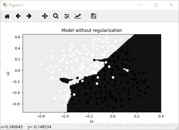
plt.title("Model without regularization")
axes = plt.gca()
axes.set_xlim([-0.75,0.40])
axes.set_ylim([-0.75,0.65])
plot_decision_boundary(lambda x: predict_dec(parameters, x.T), train_X, train_Y)

输出：

Cost after iteration 0: 0.6557412523481002
Cost after iteration 10000: 0.1632998752572419
Cost after iteration 20000: 0.13851642423239133
On the training set:
Accuracy: 0.947867298578
On the test set:
Accuracy: 0.915

2 - L2 Regularization

The standard way to avoid overfitting is called L2 regularization. It consists of appropriately modifying your cost function, from: 

输入：

parameters = model(train_X, train_Y, lambd = 0.7)
print ("On the train set:")
predictions_train = predict(train_X, train_Y, parameters)
print ("On the test set:")
predictions_test = predict(test_X, test_Y, parameters)
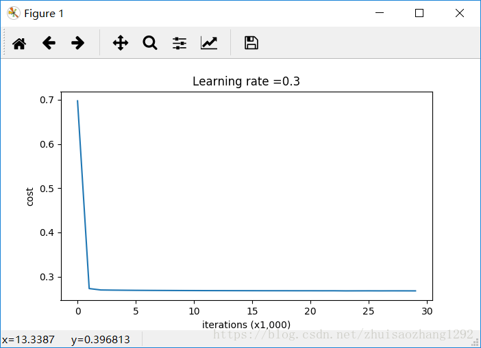
plt.title("Model with L2-regularization")
axes = plt.gca()
axes.set_xlim([-0.75,0.40])
axes.set_ylim([-0.75,0.65])
plot_decision_boundary(lambda x: predict_dec(parameters, x.T), train_X, train_Y)

输出：

Cost after iteration 0: 0.6974484493131264
Cost after iteration 10000: 0.2684918873282239
Cost after iteration 20000: 0.2680916337127301
On the train set:
Accuracy: 0.938388625592
On the test set:
Accuracy: 0.93

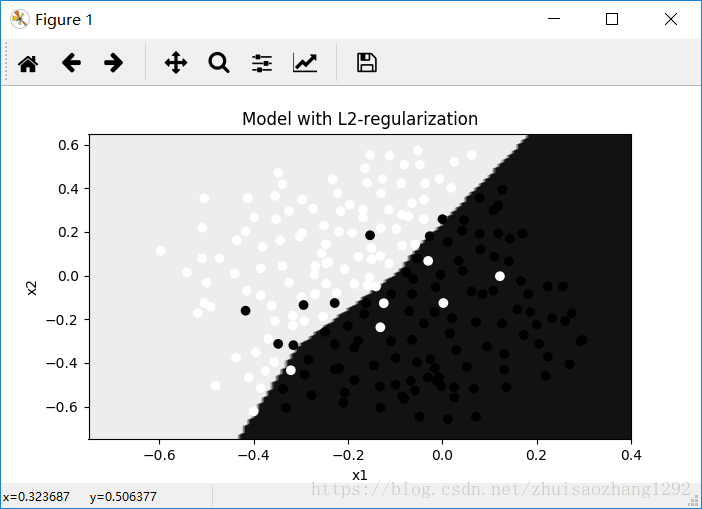
Observations: 
- The value of λλ is a hyperparameter that you can tune using a dev set.(λλ的值是一个超参数，您可以使用开发集进行调优) 
- L2 regularization makes your decision boundary smoother. If λλ is too large, it is also possible to “oversmooth”, resulting in a model with high bias.(L2正则化使得你的决策边界更加平滑。如果λλ太大，也有可能“过度平滑”，从而导致高偏差的模型)

What is L2-regularization actually doing?:

L2-regularization relies on the assumption that a model with small weights is simpler than a model with large weights. Thus, by penalizing the square values of the weights in the cost function you drive all the weights to smaller values. It becomes too costly for the cost to have large weights! This leads to a smoother model in which the output changes more slowly as the input changes. (L2规则化依赖于这样的假设，即具有小权重的模型比具有大权重的模型简单。因此，通过惩罚成本函数中权重的平方值，可以将所有权重驱动到较小的值。拥有大重量的成本太贵了！这导致更平滑的模型，其中随着输入改变，输出变化更慢)

What you should remember – the implications of L2-regularization on: 
- The cost computation: 
- A regularization term is added to the cost(正则化项被添加到代价函数中) 
- The backpropagation function: 
- There are extra terms in the gradients with respect to weight matrices(在权重矩阵的梯度中有额外的项) 
- Weights end up smaller (“weight decay”): 
- Weights are pushed to smaller values.(权重被推到较小的值)

 

3 - Dropout

Finally, dropout is a widely used regularization technique that is specific to deep learning. 
It randomly shuts down some neurons in each iteration. Watch these two videos to see what this means!(*最后，dropout是一种广泛使用的正规化技术，特定于深度学习。 
每次迭代都会随机关闭一些神经元。观看这两个视频，看看这意味着什么*)

 

Figure 2 : Drop-out on the second hidden layer. 
At each iteration, you shut down (= set to zero) each neuron of a layer with probability 1−keep_prob1−keep_prob or keep it with probability keep_probkeep_prob (50% here). The dropped neurons don’t contribute to the training in both the forward and backward propagations of the iteration.(在每一次迭代中，你关闭（=设置为零）一个层的每个神经元的概率为1−keep_prob1−keep_prob或保持它的概率 keep_probkeep_prob（这里是50％）。丢弃的神经元对迭代的向前和向后传播都没有贡献)

When you shut some neurons down, you actually modify your model. The idea behind drop-out is that at each iteration, you train a different model that uses only a subset of your neurons. With dropout, your neurons thus become less sensitive to the activation of one other specific neuron, because that other neuron might be shut down at any time. (当你关闭一些神经元时，你实际上修改了你的模型。退出背后的想法是，在每次迭代中，你都训练一个不同的模型，只使用你的神经元的一个子集。随着dropout，你的神经元因此变得不那么敏感的激活另一个特定的神经元，因为那个其他的神经元可能在任何时候被关闭)

3.1 - Forward propagation with dropout

Exercise: Implement the forward propagation with dropout. You are using a 3 layer neural network, and will add dropout to the first and second hidden layers. We will not apply dropout to the input layer or output layer. (用dropout实现前向传播。您正在使用3层神经网络，并将添加到第一个和第二个隐藏层丢失。我们不会将dropout应用到输入层或输出层)

Instructions: 
You would like to shut down some neurons in the first and second layers. To do that, you are going to carry out 4 Steps(你想关闭第一层和第二层的一些神经元。要做到这一点，你要执行4个步骤): 
1. In lecture, we dicussed creating a variable d[1]d[1] with the same shape as a[1]a[1] using np.random.rand() to randomly get numbers between 0 and 1. Here, you will use a vectorized implementation, so create a random matrix D[1]=[d[1](1)d[1](2)...d[1](m)]D[1]=[d[1](1)d[1](2)...d[1](m)] of the same dimension as A[1]A[1].(在讲座中，我们讨论了创建一个与a[1]a[1]相同的维度的变量d[1]d[1]，它使用np.random.rand（）随机获得0到1之间的数字。在这里，你将使用一个向量化的实现，所以创建一个随机矩阵D[1]=[d[1](1)d[1](2)...d[1](m)]D[1]=[d[1](1)d[1](2)...d[1](m)]与A[1]A[1]具有相同的维数) 
2. Set each entry of D[1]D[1] to be 0 with probability (1-keep_prob) or 1 with probability (keep_prob), by thresholding values in D[1]D[1] appropriately. Hint: to set all the entries of a matrix X to 0 (if entry is less than 0.5) or 1 (if entry is more than 0.5) you would do: X = (X < 0.5). Note that 0 and 1 are respectively equivalent to False and True.(通过对D[1]D[1]中的值进行阈值化，将D[1]D[1]的每个条目设置为概率（1-keep_prob）或概率为1（keep_prob）提示：要将矩阵X的所有条目设置为0（如果条目小于0.5）或1（如果条目大于0.5），您应该执行：X =（X <0.5）。请注意，0和1分别相当于False和True) 
3. Set A[1]A[1] to A[1]∗D[1]A[1]∗D[1]. (You are shutting down some neurons). You can think of D[1]D[1] as a mask, so that when it is multiplied with another matrix, it shuts down some of the values.(将A[1]A[1]设置为A[1]∗D[1]A[1]∗D[1]。 （你正在关闭一些神经元）。您可以将D[1]D[1]作为掩码，以便当它与另一个矩阵相乘时，会关闭一些值) 
4. Divide A[1]A[1] by keep_prob. By doing this you are assuring that the result of the cost will still have the same expected value as without drop-out. (This technique is also called inverted dropout.)(用keep_prob除以A[1]A[1]。通过这样做，您可以确保成本的结果仍然具有与没有退出相同的期望值。（这种技术也被称为反向丢失。）)

3.2 - Backward propagation with dropout

Exercise: Implement the backward propagation with dropout. As before, you are training a 3 layer network. Add dropout to the first and second hidden layers, using the masks D[1]D[1] and D[2]D[2] stored in the cache. (dropout的落后传播。和以前一样，你正在训练一个三层网络。使用存储在缓存中的掩码D[1]D[1] and D[2]D[2]将dropout添加到第一个和第二个隐藏层。)

Instruction: 
Backpropagation with dropout is actually quite easy. You will have to carry out 2 Steps: 
1. You had previously shut down some neurons during forward propagation, by applying a mask D[1]D[1] to A1. In backpropagation, you will have to shut down the same neurons, by reapplying the same mask D[1]D[1] to dA1. (* 
您在前向传播过程中先前已关闭了一些神经元，方法是将掩模D[1]D[1]应用于A1。在反向传播中，您必须关闭相同的神经元，方法是将相同的掩码D[1]D[1]重新应用于dA1*) 
2. During forward propagation, you had divided A1 by keep_prob. In backpropagation, you’ll therefore have to divide dA1by keep_prob again (the calculus interpretation is that if A[1]A[1] is scaled by keep_prob, then its derivative dA[1]dA[1] is also scaled by the same keep_prob).(在向前传播过程中，你用keep_prob分隔了A1。在后向传播中，你必须再次用keep_prob来分隔dA1（演算的解释是如果A[1]A[1]被keep_prob缩放，那么它的导数dA[1]dA[1]也被相同的keep_prob缩放）)

 

输入：

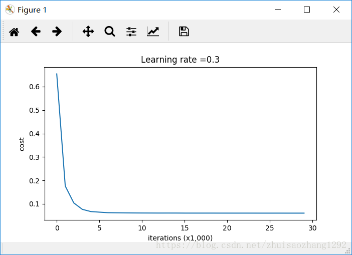
parameters = model(train_X, train_Y, keep_prob = 0.86, learning_rate = 0.3)

print ("On the train set:")
predictions_train = predict(train_X, train_Y, parameters)
print ("On the test set:")
predictions_test = predict(test_X, test_Y, parameters)
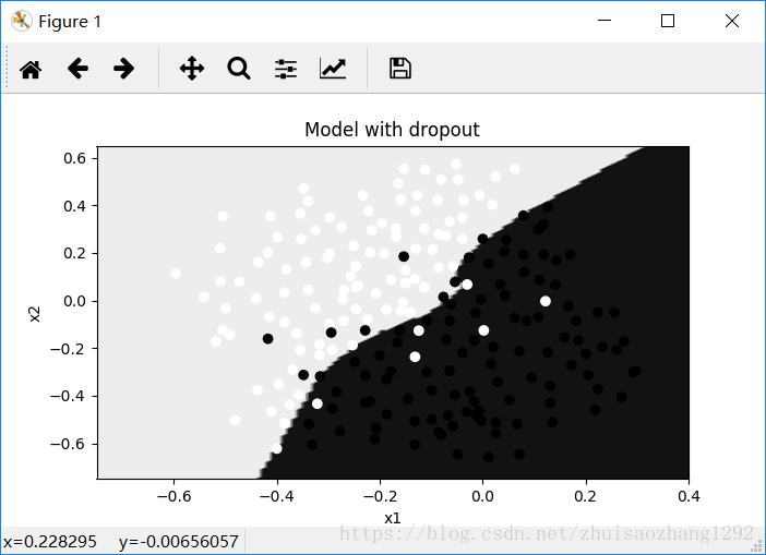
plt.title("Model with dropout")
axes = plt.gca()
axes.set_xlim([-0.75,0.40])
axes.set_ylim([-0.75,0.65])
plot_decision_boundary(lambda x: predict_dec(parameters, x.T), train_X, train_Y)

输出：

Cost after iteration 0: 0.6543912405149825
D:\F\eclipse-workspace\deep_learning\src\reg_utils.py:214: RuntimeWarning: divide by zero encountered in log
  logprobs = np.multiply(-np.log(a3),Y) + np.multiply(-np.log(1 - a3), 1 - Y)
D:\F\eclipse-workspace\deep_learning\src\reg_utils.py:214: RuntimeWarning: invalid value encountered in multiply
  logprobs = np.multiply(-np.log(a3),Y) + np.multiply(-np.log(1 - a3), 1 - Y)
Cost after iteration 10000: 0.061016986574905605
Cost after iteration 20000: 0.060582435798513114
On the train set:
Accuracy: 0.928909952607
On the test set:
Accuracy: 0.95

Note: 
- A common mistake when using dropout is to use it both in training and testing. You should use dropout (randomly eliminate nodes) only in training. (使用dropout时常见的错误是在训练和测试中使用它。你只能在训练中使用退出（随机消除节点）) 
- Deep learning frameworks like tensorflow, PaddlePaddle, keras or caffe come with a dropout layer implementation. Don’t stress - you will soon learn some of these frameworks.(深度学习框架如tensorflow，[PaddlePaddle](http://doc.paddlepaddle.org/release_doc/0.9.0/doc /ui/api/trainer_config_helpers/attrs.html)，[keras](https://keras.io/layers/core/#dropout）或[caffe]（http://caffe.berkeleyvision.org/tutorial/layers/ dropout.html)带有一个dropout层的实现。不要紧张 - 你很快就会学到一些这样的框架。)

What you should remember about dropout: 
- Dropout is a regularization technique.(droout是一种正则化技术) 
- You only use dropout during training. Don’t use dropout (randomly eliminate nodes) during test time.(训练期间只能使用dropout。测试期间不要使用dropout（随机消除节点）) 
- Apply dropout both during forward and backward propagation.(在向前和向后传播期间dropout) 
- During training time, divide each dropout layer by keep_prob to keep the same expected value for the activations. For example, if keep_prob is 0.5, then we will on average shut down half the nodes, so the output will be scaled by 0.5 since only the remaining half are contributing to the solution. Dividing by 0.5 is equivalent to multiplying by 2. Hence, the output now has the same expected value. You can check that this works even when keep_prob is other values than 0.5. (在训练时间内，通过keep_prob分隔每个丢失图层以保持激活的相同期望值。例如，如果keep_prob是0.5，那么我们将平均关闭一半的节点，所以输出将被缩放0.5，因为只剩下一半对解决方案有贡献。除以0.5相当于乘以2.因此，输出现在具有相同的期望值。即使keep_prob是0.5以外的值，你也可以检查它是否有效)

4 - Conclusions

Here are the results of our three models:

**model**	**train accuracy**	**test accuracy**
3-layer NN without regularization	95%	91.5%
3-layer NN with L2-regularization	94%	93%
3-layer NN with dropout	93%	95%

Note that regularization hurts training set performance! This is because it limits the ability of the network to overfit to the training set. But since it ultimately gives better test accuracy, it is helping your system. (* 
请注意，正规化会伤害训练集的表现！这是因为它限制了网络过度训练集的能力。但是由于它最终提供了更好的测试准确性，它正在帮助您的系统*)

Congratulations for finishing this assignment! And also for revolutionizing French football. :-)

What we want you to remember from this notebook: 
- Regularization will help you reduce overfitting. 
- Regularization will drive your weights to lower values. 
- L2 regularization and Dropout are two very effective regularization techniques.

 

附录：reg_utils.py

# -*- coding: utf-8 -*-
"""
Created on Sun Apr 22 10:52:06 2018

@author: StephenGai
"""
import numpy as np
import matplotlib.pyplot as plt
import h5py
import sklearn
import sklearn.datasets
import sklearn.linear_model
import scipy.io

def sigmoid(x):
    """
    Compute the sigmoid of x

    Arguments:
    x -- A scalar or numpy array of any size.

    Return:
    s -- sigmoid(x)
    """
    s = 1/(1+np.exp(-x))
    return s

def relu(x):
    """
    Compute the relu of x

    Arguments:
    x -- A scalar or numpy array of any size.

    Return:
    s -- relu(x)
    """
    s = np.maximum(0,x)
    
    return s

def initialize_parameters(layer_dims):
    """
    Arguments:
    layer_dims -- python array (list) containing the dimensions of each layer in our network
    
    Returns:
    parameters -- python dictionary containing your parameters "W1", "b1", ..., "WL", "bL":
                    W1 -- weight matrix of shape (layer_dims[l], layer_dims[l-1])
                    b1 -- bias vector of shape (layer_dims[l], 1)
                    Wl -- weight matrix of shape (layer_dims[l-1], layer_dims[l])
                    bl -- bias vector of shape (1, layer_dims[l])
                    
    Tips:
    - For example: the layer_dims for the "Planar Data classification model" would have been [2,2,1]. 
    This means W1's shape was (2,2), b1 was (1,2), W2 was (2,1) and b2 was (1,1). Now you have to generalize it!
    - In the for loop, use parameters['W' + str(l)] to access Wl, where l is the iterative integer.
    """  
    np.random.seed(3)
    parameters = {}
    L = len(layer_dims) # number of layers in the network

    for l in range(1, L):
        parameters['W' + str(l)] = np.random.randn(layer_dims[l], layer_dims[l-1]) / np.sqrt(layer_dims[l-1])
        parameters['b' + str(l)] = np.zeros((layer_dims[l], 1))
        
        assert(parameters['W' + str(l)].shape == layer_dims[l], layer_dims[l-1])
        assert(parameters['W' + str(l)].shape == layer_dims[l], 1)
     
    return parameters

def forward_propagation(X, parameters):
    """
    Implements the forward propagation (and computes the loss) presented in Figure 2.
    
    Arguments:
    X -- input dataset, of shape (input size, number of examples)
    parameters -- python dictionary containing your parameters "W1", "b1", "W2", "b2", "W3", "b3":
                    W1 -- weight matrix of shape ()
                    b1 -- bias vector of shape ()
                    W2 -- weight matrix of shape ()
                    b2 -- bias vector of shape ()
                    W3 -- weight matrix of shape ()
                    b3 -- bias vector of shape ()
    
    Returns:
    loss -- the loss function (vanilla logistic loss)
    """      
    # retrieve parameters
    W1 = parameters["W1"]
    b1 = parameters["b1"]
    W2 = parameters["W2"]
    b2 = parameters["b2"]
    W3 = parameters["W3"]
    b3 = parameters["b3"]
    
    # LINEAR -> RELU -> LINEAR -> RELU -> LINEAR -> SIGMOID
    Z1 = np.dot(W1, X) + b1
    A1 = relu(Z1)
    Z2 = np.dot(W2, A1) + b2
    A2 = relu(Z2)
    Z3 = np.dot(W3, A2) + b3
    A3 = sigmoid(Z3)
    
    cache = (Z1, A1, W1, b1, Z2, A2, W2, b2, Z3, A3, W3, b3)
    
    return A3, cache

def backward_propagation(X, Y, cache):
    """
    Implement the backward propagation presented in figure 2.
    
    Arguments:
    X -- input dataset, of shape (input size, number of examples)
    Y -- true "label" vector (containing 0 if cat, 1 if non-cat)
    cache -- cache output from forward_propagation()
    
    Returns:
    gradients -- A dictionary with the gradients with respect to each parameter, activation and pre-activation variables
    """
    m = X.shape[1]
    (Z1, A1, W1, b1, Z2, A2, W2, b2, Z3, A3, W3, b3) = cache
    
    dZ3 = A3 - Y
    dW3 = 1./m * np.dot(dZ3, A2.T)
    db3 = 1./m * np.sum(dZ3, axis=1, keepdims = True)
    
    dA2 = np.dot(W3.T, dZ3)
    dZ2 = np.multiply(dA2, np.int64(A2 > 0))
    dW2 = 1./m * np.dot(dZ2, A1.T)
    db2 = 1./m * np.sum(dZ2, axis=1, keepdims = True)
    
    dA1 = np.dot(W2.T, dZ2)
    dZ1 = np.multiply(dA1, np.int64(A1 > 0))
    dW1 = 1./m * np.dot(dZ1, X.T)
    db1 = 1./m * np.sum(dZ1, axis=1, keepdims = True)
    
    gradients = {"dZ3": dZ3, "dW3": dW3, "db3": db3,
                 "dA2": dA2, "dZ2": dZ2, "dW2": dW2, "db2": db2,
                 "dA1": dA1, "dZ1": dZ1, "dW1": dW1, "db1": db1}
    
    return gradients

def update_parameters(parameters, grads, learning_rate):
    """
    Update parameters using gradient descent
    
    Arguments:
    parameters -- python dictionary containing your parameters:
                    parameters['W' + str(i)] = Wi
                    parameters['b' + str(i)] = bi
    grads -- python dictionary containing your gradients for each parameters:
                    grads['dW' + str(i)] = dWi
                    grads['db' + str(i)] = dbi
    learning_rate -- the learning rate, scalar.
    
    Returns:
    parameters -- python dictionary containing your updated parameters 
    """
    n = len(parameters) // 2 # number of layers in the neural networks

    # Update rule for each parameter
    for k in range(n):
        parameters["W" + str(k+1)] = parameters["W" + str(k+1)] - learning_rate * grads["dW" + str(k+1)]
        parameters["b" + str(k+1)] = parameters["b" + str(k+1)] - learning_rate * grads["db" + str(k+1)]
        
    return parameters

def predict(X, y, parameters):
    """
    This function is used to predict the results of a  n-layer neural network.
    
    Arguments:
    X -- data set of examples you would like to label
    parameters -- parameters of the trained model
    
    Returns:
    p -- predictions for the given dataset X
    """
    m = X.shape[1]
    p = np.zeros((1,m), dtype = np.int)
    
    # Forward propagation
    a3, caches = forward_propagation(X, parameters)
    
    # convert probas to 0/1 predictions
    for i in range(0, a3.shape[1]):
        if a3[0,i] > 0.5:
            p[0,i] = 1
        else:
            p[0,i] = 0

    # print results

    #print ("predictions: " + str(p[0,:]))
    #print ("true labels: " + str(y[0,:]))
    print("Accuracy: "  + str(np.mean((p[0,:] == y[0,:]))))
    
    return p

def compute_cost(a3, Y):
    """
    Implement the cost function
    
    Arguments:
    a3 -- post-activation, output of forward propagation
    Y -- "true" labels vector, same shape as a3
    
    Returns:
    cost - value of the cost function
    """
    m = Y.shape[1]
    
    logprobs = np.multiply(-np.log(a3),Y) + np.multiply(-np.log(1 - a3), 1 - Y)
    cost = 1./m * np.nansum(logprobs)
    
    return cost

def load_dataset():
    train_dataset = h5py.File('datasets/train_catvnoncat.h5', "r")
    train_set_x_orig = np.array(train_dataset["train_set_x"][:]) # your train set features
    train_set_y_orig = np.array(train_dataset["train_set_y"][:]) # your train set labels

    test_dataset = h5py.File('datasets/test_catvnoncat.h5', "r")
    test_set_x_orig = np.array(test_dataset["test_set_x"][:]) # your test set features
    test_set_y_orig = np.array(test_dataset["test_set_y"][:]) # your test set labels

    classes = np.array(test_dataset["list_classes"][:]) # the list of classes
    
    train_set_y = train_set_y_orig.reshape((1, train_set_y_orig.shape[0]))
    test_set_y = test_set_y_orig.reshape((1, test_set_y_orig.shape[0]))
    
    train_set_x_orig = train_set_x_orig.reshape(train_set_x_orig.shape[0], -1).T
    test_set_x_orig = test_set_x_orig.reshape(test_set_x_orig.shape[0], -1).T
    
    train_set_x = train_set_x_orig/255
    test_set_x = test_set_x_orig/255

    return train_set_x, train_set_y, test_set_x, test_set_y, classes

def predict_dec(parameters, X):
    """
    Used for plotting decision boundary.
    
    Arguments:
    parameters -- python dictionary containing your parameters 
    X -- input data of size (m, K)
    
    Returns
    predictions -- vector of predictions of our model (red: 0 / blue: 1)
    """
    # Predict using forward propagation and a classification threshold of 0.5
    a3, cache = forward_propagation(X, parameters)
    predictions = (a3>0.5)
    return predictions

# def load_planar_dataset(seed):
#     
#     np.random.seed(seed)
#     
#     m = 400 # number of examples
#     N = int(m/2) # number of points per class
#     D = 2 # dimensionality
#     X = np.zeros((m,D)) # data matrix where each row is a single example
#     Y = np.zeros((m,1), dtype='uint8') # labels vector (0 for red, 1 for blue)
#     a = 4 # maximum ray of the flower
# 
#     for j in range(2):
#        
#         ix = range(N*j,N*(j+1))
#         t = np.linspace(j*3.12,(j+1)*3.12,N) + np.random.randn(N)*0.2 # theta
#         r = a*np.sin(4*t) + np.random.randn(N)*0.2 # radius
#         X[ix] = np.c_[r*np.sin(t), r*np.cos(t)]
#         Y[ix] = j
#         
#     X = X.T
#     Y = Y.T
# 
#     return X, Y

def load_planar_dataset(randomness, seed):
    
    np.random.seed(seed)
   
    m = 50
    N = int(m/2) # number of points per class
    D = 2 # dimensionality
    X = np.zeros((m,D)) # data matrix where each row is a single example
    Y = np.zeros((m,1), dtype='uint8') # labels vector (0 for red, 1 for blue)
    a = 2 # maximum ray of the flower

    for j in range(2):      
        ix = range(N*j,N*(j+1))
        if j == 0:
            t = np.linspace(j,4*3.1415*(j+1),N) #+ np.random.randn(N)*randomness # theta
            r = 0.3*np.square(t) + np.random.randn(N)*randomness # radius
        if j == 1:
            t = np.linspace(j,2*3.1415*(j+1),N) #+ np.random.randn(N)*randomness # theta
            r = 0.2*np.square(t) + np.random.randn(N)*randomness # radius         
        X[ix] = np.c_[r*np.cos(t), r*np.sin(t)]
        Y[ix] = j
        
    X = X.T
    Y = Y.T

    return X, Y

def plot_decision_boundary(model, X, y):
    # Set min and max values and give it some padding
    x_min, x_max = X[0, :].min() - 1, X[0, :].max() + 1
    y_min, y_max = X[1, :].min() - 1, X[1, :].max() + 1
    h = 0.01
    # Generate a grid of points with distance h between them
    xx, yy = np.meshgrid(np.arange(x_min, x_max, h), np.arange(y_min, y_max, h))
    # Predict the function value for the whole grid
    Z = model(np.c_[xx.ravel(), yy.ravel()])
    Z = Z.reshape(xx.shape)
    # Plot the contour and training examples
    plt.contourf(xx, yy, Z)
    plt.ylabel('x2')
    plt.xlabel('x1')
    plt.scatter(X[0, :], X[1, :], c=np.squeeze(y))
    plt.show()

def setcolor(x):
    color=[]
    for i in range(x.shape[1]):
        if x[:,i]==1:
            color.append('b')
        else:
            color.append('r')
    return color
    
def load_2D_dataset():
    data = scipy.io.loadmat('data.mat')
    train_X = data['X'].T
    train_Y = data['y'].T
    test_X = data['Xval'].T
    test_Y = data['yval'].T

    plt.scatter(train_X[0, :], train_X[1, :], c=np.squeeze(train_Y), s=40);
    
    plt.scatter(train_X[0,:], train_X[1,:], c=setcolor(train_Y), s=40)
    plt.show()
    
    return train_X, train_Y, test_X, test_Y