神经网络（1）

IBM讲神经网络的http://www.ibm.com/developerworks/cn/linux/other/l-neural/index.html

Threshold logic unit

 

这样的输入可以看成一个向量：<X ₁, X ₂, ..., X _n, theta, t>，这里 t 是一个目标或者正确分类。神经网络用这些来调整权系数，其目的使培训中的目标与其分类相匹配。权系数的调整有一个学习规则，一个理想化的学习算法如下所示：

fully_trained = FALSE
DO UNTIL (fully_trained):
    fully_trained = TRUE
    FOR EACH training_vector = <X1, X2, ..., Xn, theta, target>::
                               # Weights compared to theta
        a = (X1 * W1)+(X2 * W2)+...+(Xn * Wn) - theta
        y = sigma(a)
        IF y != target:
            fully_trained = FALSE
        FOR EACH Wi:
        MODIFY_WEIGHT(Wi)      # According to the training rule
    IF (fully_trained):
        BREAK

这是一个线性的信号分割算法，也是神经网络的基础

线性超平面的调整可以基于感知器:

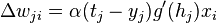
W _i 中的更改值等于 alpha * (t - y)* Xi，感性的理解是沿着X方向移动切割面，移动幅度由学习能力和误差幅度决定

也可以基于梯度，即

Delta rule

加了一项g'()，这是个梯度函数

The delta rule is derived by attempting to minimize the error in the output of the perceptron through gradient descent. The error for a perceptron with outputs can be measured as

.

In this case, we wish to move through "weight space" of the neuron (the space of all possible values of all of the neuron's weights) in proportion to the gradient of the error function with respect to each weight. In order to do that, we calculate the partial derivative of the error with respect to each weight. For the th weight, this derivative can be written as

.

Because we are only concerning ourselves with the th neuron, we can substitute the error formula above while omitting the summation:

Next we use the chain rule to split this into two derivatives:

To find the left derivative, we simply apply the general power rule:

To find the right derivative, we again apply the chain rule, this time differentiating with respect to the total input to , :

Note that the output of the neuron  is just the neuron's activation function  applied to the neuron's input . We can therefore write the derivative of  with respect to  simply as 's first derivative:

Next we rewrite  in the last term as the sum over all  weights of each weight  times its corresponding input :

Because we are only concerned with the th weight, the only term of the summation that is relevant is . Clearly,

,

giving us our final equation for the gradient:

As noted above, gradient descent tells us that our change for each weight should be proportional to the gradient. Choosing a proportionality constant  and eliminating the minus sign to enable us to move the weight in the negative direction of the gradient to minimize error, we arrive at our target equation:

.

最后这段最为重要。按梯度负方向移动，得到结果。

反向传播：

反向传播这一算法把支持 delta 规则的分析扩展到了带有隐藏节点的神经网络。为了理解这个问题，设想 Bob 给 Alice 讲了一个故事，然后 Alice 又讲给了 Ted，Ted 检查了这个事实真相，发现这个故事是错误的。现在 Ted 需要找出哪些错误是 Bob 造成的而哪些又归咎于 Alice。当输出节点从隐藏节点获得输入，网络发现出现了误差，权系数的调整需要一个算法来找出整个误差是由多少不同的节点造成的，网络需要问，“是谁让我误入歧途？到怎样的程度？如何弥补？”这时，网络该怎么做呢？

 

反向传播算法同样来源于梯度降落原理，在权系数调整分析中的唯一不同是涉及到 t(p,n) 与 y(p,n) 的差分。通常来说 W _i的改变在于：

alpha * s'(a(p,n)) * d(n) * X(p,i,n)

其中 d(n) 是隐藏节点 n 的函数，让我们来看（1）n 对任何给出的输出节点有多大影响；（2）输出节点本身对网络整体的误差有多少影响。一方面，n 影响一个输出节点越多，n 造成网络整体的误差也越多。另一方面，如果输出节点影响网络整体的误差越少，n 对输出节点的影响也相应减少。这里 d(j) 是对网络的整体误差的基值，W(n,j) 是 n 对 j 造成的影响，d(j) * W(n,j) 是这两种影响的总和。但是 n 几乎总是影响多个输出节点，也许会影响每一个输出结点，这样，d(n) 可以表示为：

SUM(d(j)*W(n,j))

这里 j 是一个从 n 获得输入的输出节点，联系起来，我们就得到了一个培训规则，第 1 部分：在隐藏节点 n 和输出节点 j 之间权系数改变，如下所示：

alpha * s'(a(p,n))*(t(p,n) - y(p,n)) * X(p,n,j)

第 2 部分：在输入节点 i 和输出节点 n 之间权系数改变，如下所示：

alpha * s'(a(p,n)) * sum(d(j) * W(n,j)) * X(p,i,n)

这里每个从 n 接收输入的输出节点 j 都不同。关于反向传播算法的基本情况大致如此。

将 Wi 初始化为小的随机值。

以下是使误差变小的迭代步骤

第 1 步：输入培训向量。  第 2 步：隐藏节点计算它们的输出  第 3 步：输出节点在第 2 步的基础上计算它们的输出。  第 4 步：计算第 3 步所得的结果和期望值之间的差。  第 5 步：把第 4 步的结果填入培训规则的第 1 部分。  第 6 步：对于每个隐藏节点 n，计算 d(n)。  第 7 步：把第 6 步的结果填入培训规则的第 2 部分。

通常把第 1 步到第 3 步称为 正向传播，把第 4 步到第 7 步称为 反向传播。反向传播的名字由此而来。