


机器学习算法与Python实践之(五)k均值聚类(k-means)
机器学习算法与Python实践这个系列主要是参考《机器学习实战》这本书。因为自己想学习Python,然后也想对一些机器学习算法加深下了解,所以就想通过Python来实现几个比较常用的机器学习算法。恰好遇见这本同样定位的书籍,所以就参考这本书的过程来学习了。
机器学习中有两类的大问题,一个是分类,一个是聚类。分类是根据一些给定的已知类别标号的样本,训练某种学习机器,使它能够对未知类别的样本进行分类。这属于supervised learning(监督学习)。而聚类指事先并不知道任何样本的类别标号,希望通过某种算法来把一组未知类别的样本划分成若干类别,这在机器学习中被称作 unsupervised learning (无监督学习)。在本文中,我们关注其中一个比较简单的聚类算法:k-means算法。
一、k-means算法
通常,人们根据样本间的某种距离或者相似性来定义聚类,即把相似的(或距离近的)样本聚为同一类,而把不相似的(或距离远的)样本归在其他类。
我们以一个二维的例子来说明下聚类的目的。如下图左所示,假设我们的n个样本点分布在图中所示的二维空间。从数据点的大致形状可以看出它们大致聚为三个cluster,其中两个紧凑一些,剩下那个松散一些。我们的目的是为这些数据分组,以便能区分出属于不同的簇的数据,如果按照分组给它们标上不同的颜色,就是像下图右边的图那样:
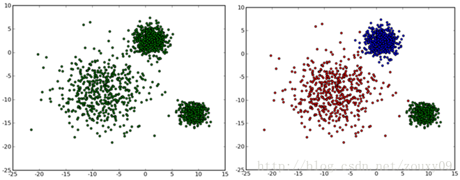
如果人可以看到像上图那样的数据分布,就可以轻松进行聚类。但我们怎么教会计算机按照我们的思维去做同样的事情呢?这里就介绍个集简单和经典于一身的k-means算法。
k-means算法是一种很常见的聚类算法,它的基本思想是:通过迭代寻找k个聚类的一种划分方案,使得用这k个聚类的均值来代表相应各类样本时所得的总体误差最小。
k-means算法的基础是最小误差平方和准则。其代价函数是:
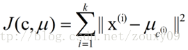
式中,μc(i)表示第i个聚类的均值。我们希望代价函数最小,直观的来说,各类内的样本越相似,其与该类均值间的误差平方越小,对所有类所得到的误差平方求和,即可验证分为k类时,各聚类是否是最优的。
上式的代价函数无法用解析的方法最小化,只能有迭代的方法。k-means算法是将样本聚类成 k个簇(cluster),其中k是用户给定的,其求解过程非常直观简单,具体算法描述如下:
1、随机选取 k个聚类质心点
2、重复下面过程直到收敛 {
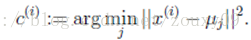
对于每一个样例 i,计算其应该属于的类:
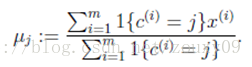
对于每一个类 j,重新计算该类的质心:
}
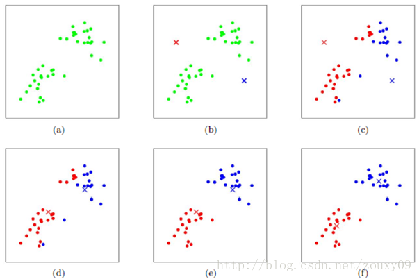
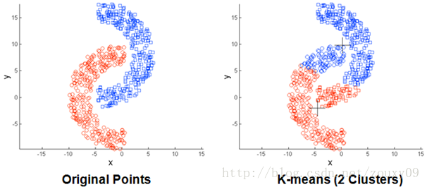
下图展示了对n个样本点进行K-means聚类的效果,这里k取2。
其伪代码如下:
********************************************************************
创建k个点作为初始的质心点(随机选择)
当任意一个点的簇分配结果发生改变时
对数据集中的每一个数据点
对每一个质心
计算质心与数据点的距离
将数据点分配到距离最近的簇
对每一个簇,计算簇中所有点的均值,并将均值作为质心
********************************************************************
二、Python实现
我使用的Python是2.7.5版本的。附加的库有Numpy和Matplotlib。具体的安装和配置见前面的博文。在代码中已经有了比较详细的注释了。不知道有没有错误的地方,如果有,还望大家指正(每次的运行结果都有可能不同)。里面我写了个可视化结果的函数,但只能在二维的数据上面使用。直接贴代码:
kmeans.py
- #################################################
- # kmeans: k-means cluster
- # Author : zouxy
- # Date : 2013-12-25
- # HomePage : http://blog.csdn.net/zouxy09
- # Email : zouxy09@qq.com
- #################################################
- from numpy import *
- import time
- import matplotlib.pyplot as plt
- # calculate Euclidean distance
- def euclDistance(vector1, vector2):
- return sqrt(sum(power(vector2 - vector1, 2)))
- # init centroids with random samples
- def initCentroids(dataSet, k):
- numSamples, dim = dataSet.shape
- centroids = zeros((k, dim))
- for i in range(k):
- index = int(random.uniform(0, numSamples))
- centroids[i, :] = dataSet[index, :]
- return centroids
- # k-means cluster
- def kmeans(dataSet, k):
- numSamples = dataSet.shape[0]
- # first column stores which cluster this sample belongs to,
- # second column stores the error between this sample and its centroid
- clusterAssment = mat(zeros((numSamples, 2)))
- clusterChanged = True
- ## step 1: init centroids
- centroids = initCentroids(dataSet, k)
- while clusterChanged:
- clusterChanged = False
- ## for each sample
- for i in xrange(numSamples):
- minDist = 100000.0
- minIndex = 0
- ## for each centroid
- ## step 2: find the centroid who is closest
- for j in range(k):
- distance = euclDistance(centroids[j, :], dataSet[i, :])
- if distance < minDist:
- minDist = distance
- minIndex = j
- ## step 3: update its cluster
- if clusterAssment[i, 0] != minIndex:
- clusterChanged = True
- clusterAssment[i, :] = minIndex, minDist**2
- ## step 4: update centroids
- for j in range(k):
- pointsInCluster = dataSet[nonzero(clusterAssment[:, 0].A == j)[0]]
- centroids[j, :] = mean(pointsInCluster, axis = 0)
- print 'Congratulations, cluster complete!'
- return centroids, clusterAssment
- # show your cluster only available with 2-D data
- def showCluster(dataSet, k, centroids, clusterAssment):
- numSamples, dim = dataSet.shape
- if dim != 2:
- print "Sorry! I can not draw because the dimension of your data is not 2!"
- return 1
- mark = ['or', 'ob', 'og', 'ok', '^r', '+r', 'sr', 'dr', '<r', 'pr']
- if k > len(mark):
- print "Sorry! Your k is too large! please contact Zouxy"
- return 1
- # draw all samples
- for i in xrange(numSamples):
- markIndex = int(clusterAssment[i, 0])
- plt.plot(dataSet[i, 0], dataSet[i, 1], mark[markIndex])
- mark = ['Dr', 'Db', 'Dg', 'Dk', '^b', '+b', 'sb', 'db', '<b', 'pb']
- # draw the centroids
- for i in range(k):
- plt.plot(centroids[i, 0], centroids[i, 1], mark[i], markersize = 12)
- plt.show()

#################################################
# kmeans: k-means cluster
# Author : zouxy
# Date   : 2013-12-25
# HomePage : http://blog.csdn.net/zouxy09
# Email  : zouxy09@qq.com
#################################################

from numpy import *
import time
import matplotlib.pyplot as plt


# calculate Euclidean distance
def euclDistance(vector1, vector2):
	return sqrt(sum(power(vector2 - vector1, 2)))

# init centroids with random samples
def initCentroids(dataSet, k):
	numSamples, dim = dataSet.shape
	centroids = zeros((k, dim))
	for i in range(k):
		index = int(random.uniform(0, numSamples))
		centroids[i, :] = dataSet[index, :]
	return centroids

# k-means cluster
def kmeans(dataSet, k):
	numSamples = dataSet.shape[0]
	# first column stores which cluster this sample belongs to,
	# second column stores the error between this sample and its centroid
	clusterAssment = mat(zeros((numSamples, 2)))
	clusterChanged = True

	## step 1: init centroids
	centroids = initCentroids(dataSet, k)

	while clusterChanged:
		clusterChanged = False
		## for each sample
		for i in xrange(numSamples):
			minDist  = 100000.0
			minIndex = 0
			## for each centroid
			## step 2: find the centroid who is closest
			for j in range(k):
				distance = euclDistance(centroids[j, :], dataSet[i, :])
				if distance < minDist:
					minDist  = distance
					minIndex = j

			## step 3: update its cluster
			if clusterAssment[i, 0] != minIndex:
				clusterChanged = True
				clusterAssment[i, :] = minIndex, minDist**2

		## step 4: update centroids
		for j in range(k):
			pointsInCluster = dataSet[nonzero(clusterAssment[:, 0].A == j)[0]]
			centroids[j, :] = mean(pointsInCluster, axis = 0)

	print 'Congratulations, cluster complete!'
	return centroids, clusterAssment

# show your cluster only available with 2-D data
def showCluster(dataSet, k, centroids, clusterAssment):
	numSamples, dim = dataSet.shape
	if dim != 2:
		print "Sorry! I can not draw because the dimension of your data is not 2!"
		return 1

	mark = ['or', 'ob', 'og', 'ok', '^r', '+r', 'sr', 'dr', '<r', 'pr']
	if k > len(mark):
		print "Sorry! Your k is too large! please contact Zouxy"
		return 1

	# draw all samples
	for i in xrange(numSamples):
		markIndex = int(clusterAssment[i, 0])
		plt.plot(dataSet[i, 0], dataSet[i, 1], mark[markIndex])

	mark = ['Dr', 'Db', 'Dg', 'Dk', '^b', '+b', 'sb', 'db', '<b', 'pb']
	# draw the centroids
	for i in range(k):
		plt.plot(centroids[i, 0], centroids[i, 1], mark[i], markersize = 12)

plt.show()三、测试结果
测试数据是二维的,共80个样本。有4个类。如下:
testSet.txt
- 1.658985 4.285136
- -3.453687 3.424321
- 4.838138 -1.151539
- -5.379713 -3.362104
- 0.972564 2.924086
- -3.567919 1.531611
- 0.450614 -3.302219
- -3.487105 -1.724432
- 2.668759 1.594842
- -3.156485 3.191137
- 3.165506 -3.999838
- -2.786837 -3.099354
- 4.208187 2.984927
- -2.123337 2.943366
- 0.704199 -0.479481
- -0.392370 -3.963704
- 2.831667 1.574018
- -0.790153 3.343144
- 2.943496 -3.357075
- -3.195883 -2.283926
- 2.336445 2.875106
- -1.786345 2.554248
- 2.190101 -1.906020
- -3.403367 -2.778288
- 1.778124 3.880832
- -1.688346 2.230267
- 2.592976 -2.054368
- -4.007257 -3.207066
- 2.257734 3.387564
- -2.679011 0.785119
- 0.939512 -4.023563
- -3.674424 -2.261084
- 2.046259 2.735279
- -3.189470 1.780269
- 4.372646 -0.822248
- -2.579316 -3.497576
- 1.889034 5.190400
- -0.798747 2.185588
- 2.836520 -2.658556
- -3.837877 -3.253815
- 2.096701 3.886007
- -2.709034 2.923887
- 3.367037 -3.184789
- -2.121479 -4.232586
- 2.329546 3.179764
- -3.284816 3.273099
- 3.091414 -3.815232
- -3.762093 -2.432191
- 3.542056 2.778832
- -1.736822 4.241041
- 2.127073 -2.983680
- -4.323818 -3.938116
- 3.792121 5.135768
- -4.786473 3.358547
- 2.624081 -3.260715
- -4.009299 -2.978115
- 2.493525 1.963710
- -2.513661 2.642162
- 1.864375 -3.176309
- -3.171184 -3.572452
- 2.894220 2.489128
- -2.562539 2.884438
- 3.491078 -3.947487
- -2.565729 -2.012114
- 3.332948 3.983102
- -1.616805 3.573188
- 2.280615 -2.559444
- -2.651229 -3.103198
- 2.321395 3.154987
- -1.685703 2.939697
- 3.031012 -3.620252
- -4.599622 -2.185829
- 4.196223 1.126677
- -2.133863 3.093686
- 4.668892 -2.562705
- -2.793241 -2.149706
- 2.884105 3.043438
- -2.967647 2.848696
- 4.479332 -1.764772
- -4.905566 -2.911070
1.658985	4.285136
-3.453687	3.424321
4.838138	-1.151539
-5.379713	-3.362104
0.972564	2.924086
-3.567919	1.531611
0.450614	-3.302219
-3.487105	-1.724432
2.668759	1.594842
-3.156485	3.191137
3.165506	-3.999838
-2.786837	-3.099354
4.208187	2.984927
-2.123337	2.943366
0.704199	-0.479481
-0.392370	-3.963704
2.831667	1.574018
-0.790153	3.343144
2.943496	-3.357075
-3.195883	-2.283926
2.336445	2.875106
-1.786345	2.554248
2.190101	-1.906020
-3.403367	-2.778288
1.778124	3.880832
-1.688346	2.230267
2.592976	-2.054368
-4.007257	-3.207066
2.257734	3.387564
-2.679011	0.785119
0.939512	-4.023563
-3.674424	-2.261084
2.046259	2.735279
-3.189470	1.780269
4.372646	-0.822248
-2.579316	-3.497576
1.889034	5.190400
-0.798747	2.185588
2.836520	-2.658556
-3.837877	-3.253815
2.096701	3.886007
-2.709034	2.923887
3.367037	-3.184789
-2.121479	-4.232586
2.329546	3.179764
-3.284816	3.273099
3.091414	-3.815232
-3.762093	-2.432191
3.542056	2.778832
-1.736822	4.241041
2.127073	-2.983680
-4.323818	-3.938116
3.792121	5.135768
-4.786473	3.358547
2.624081	-3.260715
-4.009299	-2.978115
2.493525	1.963710
-2.513661	2.642162
1.864375	-3.176309
-3.171184	-3.572452
2.894220	2.489128
-2.562539	2.884438
3.491078	-3.947487
-2.565729	-2.012114
3.332948	3.983102
-1.616805	3.573188
2.280615	-2.559444
-2.651229	-3.103198
2.321395	3.154987
-1.685703	2.939697
3.031012	-3.620252
-4.599622	-2.185829
4.196223	1.126677
-2.133863	3.093686
4.668892	-2.562705
-2.793241	-2.149706
2.884105	3.043438
-2.967647	2.848696
4.479332	-1.764772
-4.905566	-2.911070
测试代码:
test_kmeans.py
- #################################################
- # kmeans: k-means cluster
- # Author : zouxy
- # Date : 2013-12-25
- # HomePage : http://blog.csdn.net/zouxy09
- # Email : zouxy09@qq.com
- #################################################
- from numpy import *
- import time
- import matplotlib.pyplot as plt
- ## step 1: load data
- print "step 1: load data..."
- dataSet = []
- fileIn = open('E:/Python/Machine Learning in Action/testSet.txt')
- for line in fileIn.readlines():
- lineArr = line.strip().split('\t')
- dataSet.append([float(lineArr[0]), float(lineArr[1])])
- ## step 2: clustering...
- print "step 2: clustering..."
- dataSet = mat(dataSet)
- k = 4
- centroids, clusterAssment = kmeans(dataSet, k)
- ## step 3: show the result
- print "step 3: show the result..."
- showCluster(dataSet, k, centroids, clusterAssment)
#################################################
# kmeans: k-means cluster
# Author : zouxy
# Date   : 2013-12-25
# HomePage : http://blog.csdn.net/zouxy09
# Email  : zouxy09@qq.com
#################################################

from numpy import *
import time
import matplotlib.pyplot as plt

## step 1: load data
print "step 1: load data..."
dataSet = []
fileIn = open('E:/Python/Machine Learning in Action/testSet.txt')
for line in fileIn.readlines():
	lineArr = line.strip().split('\t')
	dataSet.append([float(lineArr[0]), float(lineArr[1])])

## step 2: clustering...
print "step 2: clustering..."
dataSet = mat(dataSet)
k = 4
centroids, clusterAssment = kmeans(dataSet, k)

## step 3: show the result
print "step 3: show the result..."
showCluster(dataSet, k, centroids, clusterAssment)
运行的前后结果是:
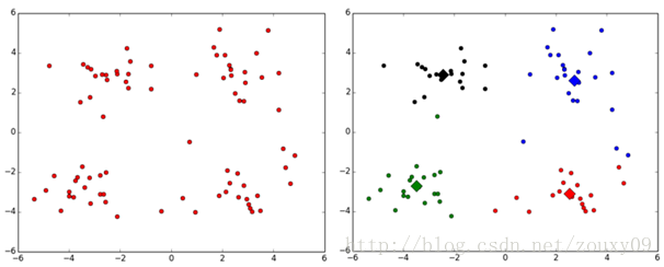
不同的类用不同的颜色来表示,其中的大菱形是对应类的均值质心点。
四、算法分析
k-means算法比较简单,但也有几个比较大的缺点:
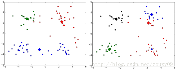
(1)k值的选择是用户指定的,不同的k得到的结果会有挺大的不同,如下图所示,左边是k=3的结果,这个就太稀疏了,蓝色的那个簇其实是可以再划分成两个簇的。而右图是k=5的结果,可以看到红色菱形和蓝色菱形这两个簇应该是可以合并成一个簇的:
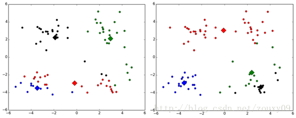
(2)对k个初始质心的选择比较敏感,容易陷入局部最小值。例如,我们上面的算法运行的时候,有可能会得到不同的结果,如下面这两种情况。K-means也是收敛了,只是收敛到了局部最小值:
(3)存在局限性,如下面这种非球状的数据分布就搞不定了:
(4)数据库比较大的时候,收敛会比较慢。
k-means老早就出现在江湖了。所以以上的这些不足也被世人的目光敏锐的捕捉到,并融入世人的智慧进行了某种程度上的改良。例如问题(1)对k的选择可以先用一些算法分析数据的分布,如重心和密度等,然后选择合适的k。而对问题(2),有人提出了另一个成为二分k均值(bisecting k-means)算法,它对初始的k个质心的选择就不太敏感,这个算法我们下一个博文再分析和实现。
五、参考文献
[1] K-means聚类算法


 23万+
23万+


 被折叠的 条评论
为什么被折叠?
被折叠的 条评论
为什么被折叠?
 到【灌水乐园】发言


