浅谈张量分解（二）：张量分解的数学基础

最新推荐文章于 2024-01-29 17:43:30 发布

zzx3163967592

最新推荐文章于 2024-01-29 17:43:30 发布

阅读量7.9k

点赞数 17

近年来，张量分解技术在数据挖掘领域得到了很好的应用，但关于张量的一些计算却与我们所熟悉的线性代数大相径庭，同时，张量计算相比以向量和矩阵计算为主导的线性代数更为抽象，这使得大量读者可能会觉得关于张量的内容很“难啃”。当然，就线性代数和多重线性代数而言，主流的观点将涉及到张量计算的内容归为“多重线性代数”（multilinear algebra，维基百科链接为：Multilinear algebra），并认为多重线性代数实际上是线性代数的延伸。

为了便于认识张量计算，这里将系统地介绍张量分解所需要的一些数学基础，该部分内容主要包括常见的Kronecker积、Khatri-Rao积、向量的外积、内积、F-范数、模态积的运算规则以及高阶奇异值分解。

1 Kronecker积

Kronecker积在张量计算中非常常见，是衔接矩阵计算和张量计算的桥梁，实际上，Kronecker积的运算规则是很简单的，给定一个大小为 $m_1\times m_2$ 的矩阵 $A$ 和一个大小为 $n_1\times n_2$ 的矩阵 $B$ ，则矩阵 $A$ 和矩阵 $B$ 的Kronecker积为

$A\otimes B = \left[ \begin{array}{cccc} a_{11}B & a_{12}B & \cdots & a_{1m_2}B \\ a_{21}B & a_{22}B & \cdots & a_{2m_2}B \\ \vdots & \vdots & \ddots & \vdots \\ a_{m_11}B & a_{m_12}B & \cdots & a_{m_1m_2}B \\ \end{array} \right]$

很明显，矩阵 $A\otimes B$ 的大小为 $\left( m_1n_1 \right) \times \left( m_2n_2 \right)$ ，即行数为 $m_1n_1$ ，列数为 $m_2n_2$ 。举一个简单的例子，给定 $A=\left[ \begin{array}{cc} 1 & 2 \\ 3 & 4 \\ \end{array} \right]$ ， $B=\left[ \begin{array}{ccc} 5 & 6 & 7\\ 8 & 9 & 10 \\ \end{array} \right]$ ，则

$A\otimes B=\left[ \begin{array}{cc} 1\times \left[ \begin{array}{ccc} 5 & 6 & 7\\ 8 & 9 & 10\\ \end{array} \right] & 2\times \left[ \begin{array}{ccc} 5 & 6 & 7\\ 8 & 9 & 10\\ \end{array} \right] \\ 3\times \left[ \begin{array}{ccc} 5 & 6 & 7\\ 8 & 9 & 10\\ \end{array} \right] & 4\times \left[ \begin{array}{ccc} 5 & 6 & 7\\ 8 & 9 & 10\\ \end{array} \right] \\ \end{array} \right]$

即 $A\otimes B=\left[ \begin{array}{cccccc} 5 & 6 & 7 & 10 & 12 & 14 \\ 8 & 9 & 10 & 16 & 18 & 20 \\ 15 & 18 & 21 & 20 & 24 & 28 \\ 24 & 27 & 30 & 32 & 36 & 40 \\ \end{array} \right]$ ，且行数为 $m_1\times n_1=2\times 2=4$ ，列数为 $m_2\times n_2=2\times 3=6$ ，其中，符号“ $\otimes$ ”表示Kronecker积。

那么，试想一下： $B\otimes A$ 与 $A\otimes B$ 是否相同呢？

$B\otimes A=\left[ \begin{array}{ccc} 5\times \left[ \begin{array}{cc} 1 & 2 \\ 3 & 4 \\ \end{array} \right] & 6\times \left[ \begin{array}{cc} 1 & 2\\ 3 & 4\\ \end{array} \right] & 7\times \left[ \begin{array}{cc} 1 & 2\\ 3 & 4\\ \end{array} \right] \\ 8\times \left[ \begin{array}{cc} 1 & 2 \\ 3 & 4 \\ \end{array} \right] & 9\times \left[ \begin{array}{cc} 1 & 2 \\ 3 & 4 \\ \end{array} \right] & 10\times \left[ \begin{array}{cc} 1 & 2\\ 3 & 4\\ \end{array} \right] \\ \end{array} \right]$

即 $B\otimes A=\left[ \begin{array}{cccccc} 5 & 10 & 6 & 12 & 7 & 14 \\ 15 & 20 & 18 & 24 & 21 & 28 \\ 8 & 16 & 9 & 18 & 10 & 20 \\ 24 & 32 & 27 & 36 & 30 & 40 \\ \end{array} \right]$ ，显然， $B\otimes A\ne A\otimes B$ .

以 $A\otimes B$ 为例，也可以考虑另外一个问题，即 $\left( A\otimes B \right) ^T=A^T\otimes B^T$ 是否成立呢？

由于 $A^T\otimes B^T=\left[ \begin{array}{cc} 1\times \left[ \begin{array}{cc} 5 & 8\\ 6 & 9\\ 7 & 10\\ \end{array} \right] & 3\times \left[ \begin{array}{cc} 5 & 8\\ 6 & 9\\ 7 & 10\\ \end{array} \right] \\ 2\times \left[ \begin{array}{cc} 5 & 8\\ 6 & 9\\ 7 & 10\\ \end{array} \right] & 4\times \left[ \begin{array}{cc} 5 & 8\\ 6 & 9\\ 7 & 10\\ \end{array} \right] \\ \end{array} \right]$ ，

即 $A^T\otimes B^T=\left[ \begin{array}{cccc} 5 & 8 & 15 & 24\\ 6 & 9 & 18 & 27\\ 7 & 10 & 21 & 30\\ 10 & 16 & 20 & 32\\ 12 & 18 & 24 & 36\\ 14 & 20 & 28 & 40\\ \end{array} \right]$ ，显然， $A^T\otimes B^T=\left( A\otimes B \right) ^T$ .

2 Khatri-Rao积

给定大小为 $m\times k$ 的矩阵 $A=\left( \vec a_1,\vec a_2,...,\vec a_k \right)$ 和大小为 $n\times k$ 的矩阵 $B=\left( \vec b_1,\vec b_2,...,\vec b_k \right)$ ，则矩阵 $A$ 和矩阵 $B$ 的Khatri-Rao积为

$A\odot B=\left( \vec a_1\otimes \vec b_1,\vec a_2\otimes \vec b_2,...,\vec a_k\otimes \vec b_k \right)$

举一个例子，给定矩阵 $A=\left[ \begin{array}{cc} 1 & 2 \\ 3 & 4 \\ \end{array} \right]=\left( \vec a_1,\vec a_2 \right)$ ， $B=\left[ \begin{array}{cc} 5 & 6 \\ 7 & 8 \\ 9 & 10 \\ \end{array} \right]=\left( \vec b_1,\vec b_2 \right)$ ，则

$A\odot B=\left( \vec a_1\otimes \vec b_1,\vec a_2\otimes \vec b_2 \right)$ $=\left[ \begin{array}{cc} \left[ \begin{array}{c} 1 \\ 3 \\ \end{array} \right]\otimes \left[ \begin{array}{c} 5 \\ 7 \\ 9 \\ \end{array} \right] & \left[ \begin{array}{c} 2 \\ 4 \\ \end{array} \right]\otimes \left[ \begin{array}{c} 6 \\ 8 \\ 10 \\ \end{array} \right] \\ \end{array} \right]$

即 $A\odot B=\left[ \begin{array}{cc} 5 & 12 \\ 7 & 16 \\ 9 & 20 \\ 15 & 24 \\ 21 & 32 \\ 27 & 40 \\ \end{array} \right]$ ，由于 $B\odot A=\left( \vec b_1\otimes \vec a_1,\vec b_2\otimes \vec a_2 \right)$ ，故 $B\odot A\ne A\odot B$ .
需要注意的是，运算符号“ $\odot$ ”不只是用来表示Khatri-Rao积，有时候也可以表示两个相同大小的矩阵的点乘（element-wise product），如给定矩阵 $A=\left[ \begin{array}{cc} 1 & 2 \\ 3 & 4 \\ \end{array} \right]$ ， $B=\left[ \begin{array}{cc} 5 & 6 \\ 7 & 8 \\ \end{array} \right]$ ，则

$A\odot B=A.*B=\left[ \begin{array}{cc} 1\times 5 & 2\times 6 \\ 3\times 7 & 4\times 8 \\ \end{array} \right]=\left[ \begin{array}{cc} 5 & 12 \\ 21 & 32 \\ \end{array} \right]$ .

3 向量的外积（vector outer product）

给定向量 $\vec a=\left( 1,2 \right) ^{T}$ ，向量 $\vec b=\left( 3,4 \right) ^{T}$ ，则 $\vec a\circ \vec b=\vec a\vec b^{T}=\left[ \begin{array}{cc} 3 & 4 \\ 6 & 8 \\ \end{array} \right]$ ，运算符号“ $\circ$ ”表示外积。另给定向量 $\vec c=\left( 5,6,7 \right) ^{T}$ ，若 ${\mathcal{X}}=\vec a\circ \vec b\circ \vec c$ ，则

${\mathcal{X}}\left( :,:,1\right) =\left[ \begin{array}{cc} 1\times 3\times 5 & 1\times 4\times 5 \\ 2\times 3\times 5 & 2\times 4\times 5 \\ \end{array} \right]=\left[ \begin{array}{cc} 15 & 20 \\ 30 & 40 \\ \end{array} \right]$ ，

${\mathcal{X}}\left( :,:,2\right) =\left[ \begin{array}{cc} 1\times 3\times 6 & 1\times 4\times 6 \\ 2\times 3\times 6 & 2\times 4\times 6 \\ \end{array} \right]=\left[ \begin{array}{cc} 18 & 24 \\ 36 & 48 \\ \end{array} \right]$ ，

${\mathcal{X}}\left( :,:,3\right) =\left[ \begin{array}{cc} 1\times 3\times 7 & 1\times 4\times 7 \\ 2\times 3\times 7 & 2\times 4\times 7 \\ \end{array} \right]=\left[ \begin{array}{cc} 21 & 28 \\ 42 & 56 \\ \end{array} \right]$ ，

其中， ${\mathcal{X}}$ 是一个三维数组（有三个索引），对于任意索引 $\left( i,j,k \right)$ 上的值为 $x_{ijk}=a_i\cdot b_j\cdot c_k,i=1,2,j=1,2,k=1,2,3$ ，在这里，向量 $\vec a$ , $\vec b$ , $\vec c$ 的外积即可得到一个第三阶张量（third-order tensor），如图1所示。

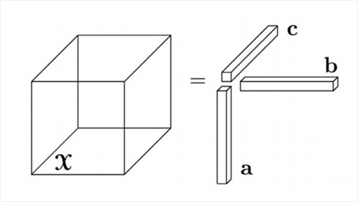
图1 向量 $\vec a$ , $\vec b$ , $\vec c$ 的外积

在大量的文献中，Kronecker积的符号“ $\otimes$ ”有时也用来表示向量的外积。

4 内积（inner product）

众所周知，向量的内积是一个标量，如给定向量 $\vec a=\left( 1,2 \right) ^{T}$ ，向量 $\vec b=\left( 3,4 \right) ^{T}$ ，则向量 $\vec a$ , $\vec b$ 的内积为

$\left<\vec a,\vec b\right>=\vec a^T\vec b=1\times 3+2\times 4=11$

当给定两个大小相同的第三阶张量 ${\mathcal{X}}$ 和 ${\mathcal{ Y}}$ ，如 ${\mathcal{ X}}\left( :,:,1 \right) =\left[ \begin{array}{cc} 1 & 2 \\ 3 & 4 \\ \end{array} \right]$ ， ${\mathcal{ X}}\left( :,:,2 \right) =\left[ \begin{array}{cc} 5 & 6 \\ 7 & 8 \\ \end{array} \right]$ ， ${\mathcal{ Y}}\left( :,:,1 \right) =\left[ \begin{array}{cc} 9 & 10 \\ 11 & 12 \\ \end{array} \right]$ ， ${\mathcal{ Y}}\left( :,:,2 \right) =\left[ \begin{array}{cc} 13 & 14 \\ 15 & 16 \\ \end{array} \right]$ ，则

$\left<{\mathcal{ X}},{\mathcal{ Y}}\right>=1\times 9+2\times 10+3\times 11+4\times 12$ $+5\times 13+6\times 14+7\times 15+8\times 16=492$ .

即两个大小相同的张量其内积是一个标量，这可能也是内积有时候被称为标量积（scalar product）的原因。

5 F-范数（Frobenius norm）

给定张量 ${\mathcal{ X}}$ 为 ${\mathcal{ X}}\left( :,:,1 \right) =\left[ \begin{array}{cc} 1 & 2 \\ 3 & 4 \\ \end{array} \right]$ ， ${\mathcal{ X}}\left( :,:,2 \right) =\left[ \begin{array}{cc} 5 & 6 \\ 7 & 8 \\ \end{array} \right]$ ，则该张量的F-范数为

$||{\mathcal{ X}}||_F=\sqrt{\left<{\mathcal{ X}},{\mathcal{ X}}\right>}$ $=\sqrt{1^2+2^2+3^2+4^2+5^2+6^2+7^2+8^2} =\sqrt{204}$

即张量 ${\mathcal{ X}}$ F-范数的平方等于其所有元素的平方和，正是这样，很多涉及到矩阵分解或张量分解的优化问题中常常会出现残差矩阵的平方和最小化或是残差张量的平方和最小化，目标函数也多以相应的残差矩阵或残差张量的F-范数的平方形式进行书写。

6 张量的展开（unfolding）

在实际应用中，由于高阶张量比向量、矩阵都抽象，最简单地，向量和矩阵可以很轻松地书写出来并进行运算，而高阶张量则不那么直观，如何将高阶张量转换成二维空间的矩阵呢？这就是张量的展开，有时，也将张量的展开称为张量的矩阵化（Matricization: transforming a tensor into a matrix）。

给定大小为 $4\times 3\times 2$ 的张量 ${\mathcal{ X}}$ ，其中，矩阵 ${\mathcal{ X}}\left( :,:,1 \right)= \left[ \begin{array}{ccc} x_{111} & x_{121} & x_{131} \\ x_{211} & x_{221} & x_{231} \\ x_{311} & x_{321} & x_{331} \\ x_{411} & x_{421} & x_{431} \\ \end{array} \right]$ ，矩阵 ${\mathcal{ X}}\left( :,:,2 \right)= \left[ \begin{array}{ccc} x_{112} & x_{122} & x_{132} \\ x_{212} & x_{222} & x_{232} \\ x_{312} & x_{322} & x_{332} \\ x_{412} & x_{422} & x_{432} \\ \end{array} \right]$ ，按照模态1（mode-1, 即对应着张量的第一阶）展开可以得到，

${\mathcal{ X}}_{\left( 1 \right) }=\left[ \begin{array}{cccccc} x_{111} & x_{121} & x_{131} & x_{112} & x_{122} & x_{132} \\ x_{211} & x_{221} & x_{231} & x_{212} & x_{222} & x_{232} \\ x_{311} & x_{321} & x_{331} & x_{312} & x_{322} & x_{332} \\ x_{411} & x_{421} & x_{431} & x_{412} & x_{422} & x_{432} \\ \end{array} \right]$

即矩阵 ${\mathcal{ X}}_{\left( 1 \right)} =\left[{\mathcal{ X}}\left( :,:,1 \right) ,{\mathcal{ X}}\left( :,:,2 \right) \right]$ ，其大小为 $4\times 6$ .

按照模态2（mode-2, 即对应着张量的第二阶）展开可以得到，

${\mathcal{ X}}_{\left( 2 \right) }=\left[ \begin{array}{ccccccccc} x_{111} & x_{211} & x_{311} & x_{411} & x_{112} & x_{212} & x_{312} & x_{412} \\ x_{121} & x_{221} & x_{321} & x_{421} & x_{122} & x_{222} & x_{322} & x_{422} \\ x_{131} & x_{231} & x_{331} & x_{431} & x_{132} & x_{232} & x_{332} & x_{432} \\ \end{array} \right]$

即矩阵 ${\mathcal{ X}}_{\left( 2 \right) }=\left[{\mathcal{ X}}\left( :,:,1 \right)^T,{\mathcal{ X}}\left( :,:,2 \right)^T \right]$ ，其大小为 $3\times 8$ .

按照模态3（mode-3, 即对应着张量的第三阶）展开可以得到，

${\mathcal{ X}}_{\left( 3 \right) }=\left[ \begin{array}{ccccccccccccc} x_{111} & x_{211} & x_{311} & x_{411} & x_{121} & x_{221} & x_{321} & x_{421} & x_{131} & x_{231} & x_{331} & x_{431} \\ x_{112} & x_{212} & x_{312} & x_{412} & x_{122} & x_{222} & x_{322} & x_{422} & x_{132} & x_{232} & x_{332} & x_{432} \\ \end{array} \right]$

即矩阵 ${\mathcal {X}}_{\left( 3 \right) }=\left[{\mathcal{ X}}\left( :,1,: \right)^T,{\mathcal{ X}}\left( :,2,: \right)^T,{\mathcal{ X}}\left( :,3,: \right)^T \right]$ ，其大小为 $2\times 12$ .

类似地，如果给定一个大小为 $2\times 2\times 2\times 2$ 的第四阶张量 ${\mathcal{ X}}$ ，则在各个模态下的展开分别为

${\mathcal{ X}}_{\left( 1 \right) }=\left[{\mathcal{ X}}\left( :,:,1,1 \right),{\mathcal{ X}}\left( :,:,2,1 \right),{\mathcal{ X}}\left( :,:,1,2 \right),{\mathcal{ X}}\left( :,:,2,2 \right) \right]$ ，

${\mathcal{ X}}_{\left( 2 \right) }=\left[{\mathcal{ X}}\left( :,:,1,1 \right)^T,{\mathcal{ X}}\left( :,:,2,1 \right)^T,{\mathcal{ X}}\left( :,:,1,2 \right)^T,{\mathcal{ X}}\left( :,:,2,2 \right)^T \right]$ ，

${\mathcal{ X}}_{\left( 3 \right) }=\left[{\mathcal{ X}}\left( :,1,:,1 \right)^T,{\mathcal{ X}}\left( :,2,:,1 \right)^T,{\mathcal{ X}}\left( :,1,:,2 \right)^T,{\mathcal{ X}}\left( :,2,:,2 \right)^T \right]$ ，

${\mathcal{ X}}_{\left( 4 \right) }=\left[{\mathcal{ X}}\left( :,1,1,: \right)^T,{\mathcal{ X}}\left( :,2,1,: \right)^T,{\mathcal{ X}}\left( :,1,2,: \right)^T,{\mathcal{ X}}\left( :,2,2,: \right)^T \right]$ .

举一个例子，若 ${\mathcal{ X}}\left( :,:,1,1 \right) =\left[ \begin{array}{cc} 1 & 2 \\ 3 & 4 \\ \end{array} \right]$ ， ${\mathcal{ X}}\left( :,:,2,1 \right) =\left[ \begin{array}{cc} 5 & 6 \\ 7 & 8 \\ \end{array} \right]$ ， ${\mathcal{ X}}\left( :,:,1,2 \right) =\left[ \begin{array}{cc} 9 & 10 \\ 11 & 12 \\ \end{array} \right]$ ， ${\mathcal{ X}}\left( :,:,2,2 \right) =\left[ \begin{array}{cc} 13 & 14 \\ 15 & 16 \\ \end{array} \right]$ ，则

${\mathcal{ X}}_{\left( 1 \right) } =\left[ \begin{array}{cccccccc} 1 & 2 & 5 & 6 & 9 & 10 & 13 & 14 \\ 3 & 4 & 7 & 8 & 11 & 12 & 15 & 16 \\ \end{array} \right]$ ，

${\mathcal{ X}}_{\left( 2 \right) } =\left[ \begin{array}{cccccccc} 1 & 3 & 5 & 7 & 9 & 11 & 13 & 15 \\ 2 & 4 & 6 & 8 & 10 & 12 & 14 & 16 \\ \end{array} \right]$ ，

${\mathcal{ X}}_{\left( 3 \right) } =\left[ \begin{array}{cccccccc} 1 & 3 & 2 & 4 & 9 & 11 & 10 & 12 \\ 5 & 7 & 6 & 8 & 13 & 15 & 14 & 16 \\ \end{array} \right]$ ，

${\mathcal{ X}}_{\left( 4 \right) } =\left[ \begin{array}{cccccccc} 1 & 3 & 2 & 4 & 5 & 7 & 6 & 8 \\ 9 & 11 & 10 & 12 & 13 & 15 & 14 & 16 \\ \end{array} \right]$ .

可惜的是，张量的展开虽然有一定的规则，但并没有很强的物理意义，对高阶张量进行展开会方便使用相应的矩阵化运算。除此之外，高阶张量可以展开自然也就可以还原（即将展开后的矩阵还原成高阶张量，这个过程称为folding）。

7 张量与矩阵相乘（modal product, 模态积）

张量与矩阵相乘（又称为模态积）相比矩阵与矩阵之间的相乘更为抽象，如何理解呢？

假设一个大小为 $n_1 \times n_2 \times ... \times n_d$ 的张量 ${\mathcal{X}}$ ，同时给定一个大小为 $m\times n_k$ 的矩阵 $A$ ，则张量 ${\mathcal{X}}$ 与矩阵 $A$ 的 $k$ 模态积（ $k$ -mode product）记为 ${\mathcal{X}}\times_k A$ ，其大小为 $n_1 \times n_2 \times ... \times n_{k-1} \times m \times n_{k+1} \times ... \times n_d$ ，对于每个元素而言，有

$\left({\mathcal{X}}\times_k A \right) _{i_1i_2...i_{k-1}ji_{k+1}...i_d}=\sum_{i_k=1}^{n_k}{x_{i_1i_2...i_d}a_{ji_k}}$

其中， $1\leq i_1\leq n_1,...,1\leq i_d\leq n_d,1\leq j\leq m$ ，我们可以看出，模态积是张量、矩阵和模态（mode）的一种“组合”运算。另外， ${\mathcal{Y}}={\mathcal{X}}\times_kA$ 与 ${\mathcal{Y}}_{\left( k \right) }=A{\mathcal{X}}_{\left( k \right) }$ 是等价的，这在接下来的例子里会展现相应的计算过程。

上述给出张量与矩阵相乘的定义，为了方便理解，下面来看一个简单的示例，若给定张量 ${\mathcal{ X}}$ 为 ${\mathcal{ X}}\left( :,:,1 \right) =\left[ \begin{array}{cc} 1 & 2 \\ 3 & 4 \\ \end{array} \right]$ ， ${\mathcal{ X}}\left( :,:,2 \right) =\left[ \begin{array}{cc} 5 & 6 \\ 7 & 8 \\ \end{array} \right]$ ，其大小为 $2\times 2\times 2$ ，另外给定矩阵 $A=\left[ \begin{array}{cc} 1 & 2 \\ 3 & 4 \\ 5 & 6 \\ \end{array} \right]$ ，试想一下：张量 ${\mathcal{ X}}$ 和矩阵 $A$ 相乘会得到什么呢？

假设 ${\mathcal{ Y}}={\mathcal{ X}}\times _1A$ ，则对于张量 ${\mathcal{ Y}}$ 在任意索引 $\left( i,j,k \right)$ 上的值为 $y_{ijk}=\sum_{m=1}^{2}{\left( x_{mjk}\cdot a_{im} \right) }$ ，这一运算规则也不难发现，张量 ${\mathcal{ Y}}$ 的大小为 $3\times 2\times 2$ ，以 $\left( 1,1,1 \right)$ 位置为例， $y_{111}=\sum_{m=1}^{2}{\left( x_{m11}\cdot a_{1m} \right) } =x_{111}\cdot a_{11}+x_{211}\cdot a_{12}=7$

再以 $\left( 1,1,2 \right)$ 位置为例， $y_{112}=\sum_{m=1}^{2}{\left( x_{m12}\cdot a_{1m} \right) }$ $=x_{112}\cdot a_{11}+x_{212}\cdot a_{12}=19$ ，这样，可以得到张量 ${\mathcal{ Y}}$ 为

${\mathcal{ Y}}\left( :,:,1 \right) =\left[ \begin{array}{cc} x_{111} a_{11}+x_{211} a_{12} & x_{121} a_{11}+x_{221} a_{12} \\ x_{111} a_{21}+x_{211} a_{22} & x_{121} a_{21}+x_{221} a_{22} \\ x_{111} a_{31}+x_{211} a_{32} & x_{121} a_{31}+x_{221} a_{32} \\ \end{array} \right]$ ，

${\mathcal{ Y}}\left( :,:,2 \right) =\left[ \begin{array}{cc} x_{112} a_{11}+x_{212} a_{12} & x_{122} a_{11}+x_{222} a_{12} \\ x_{112} a_{21}+x_{212} a_{22} & x_{122} a_{21}+x_{222} a_{22} \\ x_{112} a_{31}+x_{212} a_{32} & x_{122} a_{31}+x_{222} a_{32} \\ \end{array} \right]$ ，

即 ${\mathcal{ Y}}\left( :,:,1 \right) =\left[ \begin{array}{cc} 1\times 1+3\times 2 & 2\times 1+4\times 2 \\ 1\times 3+3\times 4 & 2\times 3+4\times 4 \\ 1\times 5+3\times 6 & 2\times 5+4\times 6 \\ \end{array} \right]=\left[ \begin{array}{cc} 7 & 10 \\ 15 & 22 \\ 23 & 34 \\ \end{array} \right]$ ， ${\mathcal{ Y}}\left( :,:,2 \right) =\left[ \begin{array}{cc} 5\times 1+7\times 2 & 6\times 1+8\times 2 \\ 5\times 3+7\times 4 & 6\times 3+8\times 4 \\ 5\times 5+7\times 6 & 6\times 5+8\times 6 \\ \end{array} \right]=\left[ \begin{array}{cc} 19 & 22 \\ 43 & 50 \\ 67 & 78 \\ \end{array} \right]$ .

其中，由于模态积的运算规则不再像Kronecer积和Khatri-Rao积那么“亲民”，所以有兴趣的读者可以自己动手计算一遍。

实际上， ${\mathcal{ Y}}={\mathcal{ X}}\times _2A$ （会得到大小为 $2\times 3\times 2$ 的张量）或 ${\mathcal{ Y}}={\mathcal{ X}}\times _3A$ （会得到大小为 $2\times 2\times 3$ 的张量）也可以用上述同样的运算规则进行计算，这里将不再赘述，有兴趣的读者可以自行推导。需要注意的是， ${\mathcal{ Y}}={\mathcal{ X}}\times _1A$ 有一个恒等的计算公式，即 ${\mathcal{ Y}}_{\left( 1 \right) }=A{\mathcal{ X}}_{\left( 1 \right) }$ ，由于 ${\mathcal{ X}}_{\left( 1 \right) }=\left[{\mathcal{ X}}\left( :,:,1 \right) ,{\mathcal{ X}}\left( :,:,2 \right) \right] =\left[ \begin{array}{cccc} 1 & 2 & 5 & 6 \\ 3 & 4 & 7 & 8 \\ \end{array} \right]$ ，则

${\mathcal{ Y}}_{\left( 1 \right) }=\left[ \begin{array}{cccc} 7 & 10 & 19 & 22 \\ 15 & 22 & 43 & 50 \\ 23 & 34 & 67 & 78 \\ \end{array} \right]$

满足 ${\mathcal{ Y}}_{\left( 1 \right) }=\left[{\mathcal{ Y}}\left( :,:,1 \right) ,{\mathcal{ Y}}\left( :,:,2 \right) \right]$ ，即采用张量矩阵化的形式进行运算可以使问题变得更加简单，从这里也可以看出高阶张量进行矩阵化的优点。

8 延伸阅读：高阶奇异值分解（higher-order singular value decomposition, 简称HOSVD）

矩阵的奇异值分解（singular value decomposition，简称SVD）是线性代数中很重要的内容，通常，给定一个大小为 $m\times n$ 的矩阵 $A$ ，奇异值分解的形式为

$A=U\Sigma V^T$

其中，矩阵 $U,\Sigma,V$ 的大小分别为 $m\times m,m\times n,n\times n$ ，矩阵 $U$ 是由左奇异向量（left singular vector）构成的，矩阵 $V$ 是由右奇异向量（right singular vector）构成的，矩阵 $\Sigma$ 对角线上的元素称为奇异值（singular value），这一分解过程很简单，但实际上，关于奇异值分解的应用是非常广泛的。

就高阶奇异值分解而言，著名学者Tucker于1966年给出了计算Tucker分解的三种方法，第一种方法就是我们这里要提到的高阶奇异值分解，其整个分解过程也是由矩阵的奇异值分解泛化得到的。

对于给定一个大小为 $n_1 \times n_2 \times ... \times n_d$ 的张量 ${\mathcal{X}}$ ，将 $k$ 模态下的展开记为 ${\mathcal{X}}_{\left( k \right) }$ ，则 $k$ 模态的矩阵进行奇异值分解，可以写成

${\mathcal{X}}_{\left( k \right) }=U_k\Sigma_kV_k^T,k=1,2,...,d$

这里的 $U_k,\Sigma_k,V_k$ 是通过矩阵 ${\mathcal{X}}_{\left( k \right) }$ 的奇异值分解得到的，如果取出各个模态下得到的矩阵 $U_1,U_2,...,U_d$ ，则张量 ${\mathcal{X}}$ 的高阶奇异值分解可以写成如下形式：

${\mathcal{X}}={\mathcal{G}} \times_1U_1 \times_2U_2... \times_dU_d$

其中， ${\mathcal{G}}$ 是核心张量，其计算公式为 ${\mathcal{G}}={\mathcal{X}} \times_1U_1^T \times_2U_2^T... \times_dU_d^T$ ，在这里，这条计算公式等价于 ${\mathcal{G}}_{\left( k \right) }=U_k^T{\mathcal{X}}_{\left( k \right) }\left( U_d \otimes ... \otimes U_{k+1} \otimes U_{k-1} \otimes... \otimes U_1 \right)$ （ ${\mathcal{X}}_{\left( k \right) }=U_k{\mathcal{G}}_{\left( k \right) }\left( U_d \otimes ... \otimes U_{k+1} \otimes U_{k-1} \otimes... \otimes U_1 \right)^T$ 也是恒成立的）。

细心的读者可能会发现，根据奇异值分解的定义，这里的核心张量 ${\mathcal{G}}$ 的大小为 $n_1\times n_2\times\cdots\times n_d$ ，而矩阵 $U_1,U_2,...,U_d$ 的大小则分别为 $n_1\times n_1,n_2\times n_2,...,n_d \times n_d$ .

我们也知道，对于矩阵的奇异值分解是可以进行降维（dimension reduction）处理的，即取前 $r$ 个最大奇异值以及相应的左奇异向量和右奇异向量，我们可以得到矩阵 $U,\Sigma,V$ 的大小分别为 $m\times r,r\times r,n\times r$ ，这也被称为截断的奇异值分解（truncated SVD），对于高阶奇异值分解是否存在类似的“降维”过程（即truncated HOSVD, 截断的高阶奇异值分解）呢？

给定核心张量 ${\mathcal{G}}$ 的大小为 $r_1 \times r_2 \times ... \times r_d$ ，并且 $r_1\leq n_1$ , $r_2\leq n_2$ ,..., $r_d\leq n_d$ ，则对于 $k$ 模态的矩阵 ${\mathcal{X}}_{\left( k \right) }$ 进行奇异值分解取前 $r_k$ 个最大奇异值对应的左奇异向量，则矩阵 $U_k$ 的大小为 $n_k\times r_k$ ，对矩阵 ${\mathcal{X}}_{\left( k \right) },k=1,2,...,d$ 进行奇异值分解，知道了 $U_1,U_2,...,U_d$ 后，再计算核心张量 ${\mathcal{G}}={\mathcal{X}} \times_1U_1^T \times_2U_2^T... \times_dU_d^T$ ，我们就可以最终得到想要的Tucker分解了。

9 相关阅读

本文主要参考了Gene H. Golub和Charles F. Van Loan合著的经典著作《Matrix computations (4th edition)》，有兴趣的读者可以阅读第12章的12.3 Kronecker Product Computations, 12.4 Tensor Unfoldings and Contractions和12.5 Tensor Decompositions and Iterations；另外，Tamara G. Kolda和Brett W. Bader于2009年发表的一篇经典综述论文《Tensor decompositions and Applications》（链接为：http://public.ca.sandia.gov/~tgkolda/pubs/pubfiles/TensorReview.pdf）也是本文的主要参考资料。

zzx3163967592

关注

17
点赞
踩
105

收藏

觉得还不错? 一键收藏
2
评论
浅谈张量分解（二）：张量分解的数学基础

近年来，张量分解技术在数据挖掘领域得到了很好的应用，但关于张量的一些计算却与我们所熟悉的线性代数大相径庭，同时，张量计算相比以向量和矩阵计算为主导的线性代数更为抽象，这使得大量读者可能会觉得关于张量的内容很“难啃”。当然，就线性代数和多重线性代数而言，主流的观点将涉及到张量计算的内容归为“多重线性代数”（multilinear algebra，维基百科链接为：Multilinear algebra...
复制链接

扫一扫