概述
本文使用Kaggle上的一个公开数据集,从数据导入,清理整理一直介绍到最后数据多个算法建模,交叉验证以及多个预测模型的比较全过程,注重在实际数据建模过程中的实际问题和挑战,主要包括以下五个方面的挑战:
- 缺失值的挑战
- 异常值的挑战
- 不均衡分布的挑战
- (多重)共线性的挑战
- 预测因子的量纲差异
以上的几个主要挑战,对于熟悉机器学习的人来说,应该都是比较清楚的,这个案例中会涉及到五个挑战中的缺失值,量纲和共线性问题的挑战。
案例数据说明
本案例中的数据可以在下面的网址中下载:
https://www.kaggle.com/primaryobjects/voicegender/downloads/voicegender.zip
下载到本地后解压缩会生成voice.csv文件
下面首先大概了解一下我们要用来建模的数据
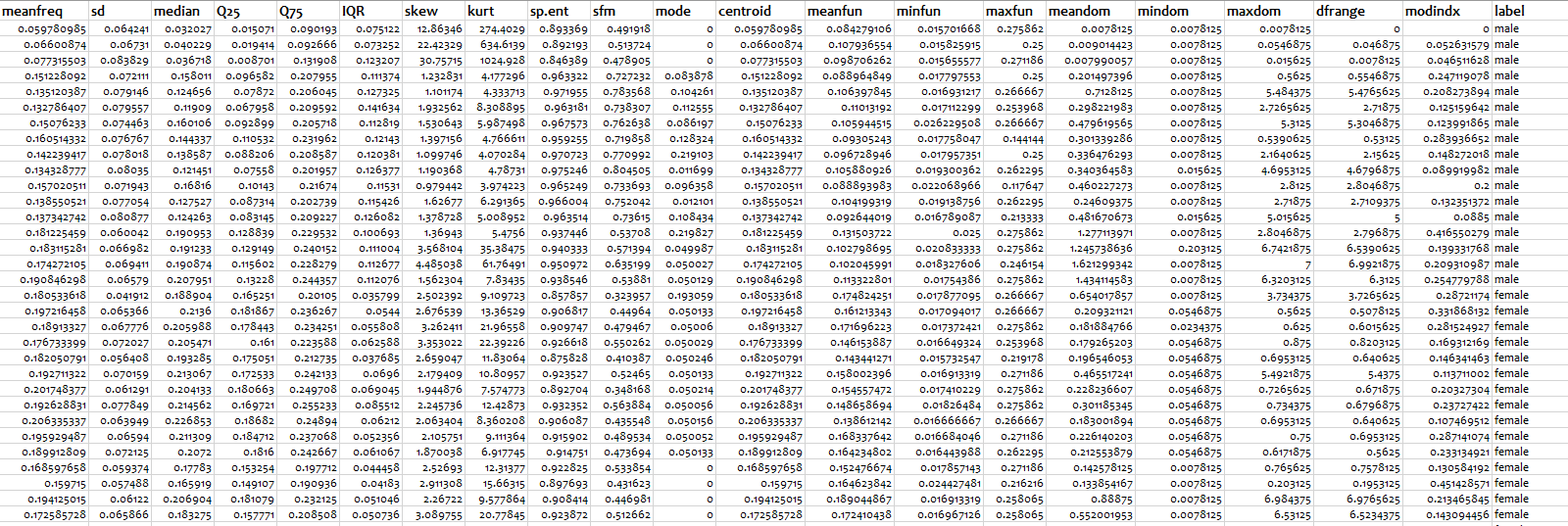
数据共包含21个变量,最后一个变量label是需要我们进行预测的变量,即性别是男或者女
前面20个变量都是我们的预测因子,每一个都是用来描述声音的量化属性。
下面我们开始我们的具体过程
步骤1:基本准备工作
步骤1主要包含以下三项工作:
- 设定工作目录
- 载入需要使用的包
- 准备好并行计算
setwd("C:/Users/chn-fzj/Desktop/R Projects/Kaggle-Gender by Voice")
require(readr)
require(ggplot2)
require(dplyr)
require(tidyr)
require(caret)
require(corrplot)
require(Hmisc)
require(parallel)
require(doParallel)
require(ggthemes)
n_Cores <- detectCores()
cluster_Set <- makeCluster(n_Cores)
registerDoParallel(cluster_Set)
- 1
- 2
- 3
- 4
- 5
- 6
- 7
- 8
- 9
- 10
- 11
- 12
- 13
- 14
- 15
- 16
- 17
- 18
- 19
- 20
- 1
- 2
- 3
- 4
- 5
- 6
- 7
- 8
- 9
- 10
- 11
- 12
- 13
- 14
- 15
- 16
- 17
- 18
- 19
- 20
步骤2:数据的导入和理解
数据下载解压缩后就是一份名为‘voice.csv’ 的文件,我们将csv文件存到我们设定的工作目录之中,就可以导入数据了。
voice_Original <- read_csv("voice.csv",col_names=TRUE)
describe(voice_Original)
Hmisc包中的describe 函数是我个人最喜欢的对数据集进行概述,整体上了解数据集的最好的一个函数,运行结果如下:
voice_Original
meanfreq
n missing unique Info Mean .05 .10 .25
3168 0 3166 1 0.1809 0.1260 0.1411 0.1637
.50 .75 .90 .95
0.1848 0.1991 0.2177 0.2291
lowest : 0.03936 0.04825 0.05965 0.05978 0.06218
sd
n missing unique Info Mean .05 .10 .25
3168 0 3166 1 0.05713 0.03162 0.03396 0.04195
.50 .75 .90 .95
0.05916 0.06702 0.07966 0.08549
lowest : 0.01836 0.02178 0.02400 0.02427 0.02456
median
n missing unique Info Mean .05 .10 .25
3168 0 3077 1 0.1856 0.1164 0.1340 0.1696
.50 .75 .90 .95
0.1900 0.2106 0.2274 0.2358
lowest : 0.01097 0.01359 0.01579 0.02699 0.02936
Q25
n missing unique Info Mean .05 .10 .25
3168 0 3103 1 0.1405 0.04358 0.07509 0.11109
.50 .75 .90 .95
0.14029 0.17594 0.20063 0.21524
lowest : 0.0002288 0.0002355 0.0002395 0.0002502 0.0002669
Q75
n missing unique Info Mean .05 .10 .25
3168 0 3034 1 0.2248 0.1874 0.1963 0.2087
.50 .75 .90 .95
0.2257 0.2437 0.2536 0.2577
lowest : 0.04295 0.05827 0.07596 0.09019 0.09267
IQR
n missing unique Info Mean .05 .10 .25
3168 0 3073 1 0.08431 0.02549 0.02931 0.04256
.50 .75 .90 .95
0.09428 0.11418 0.13284 0.15632
lowest : 0.01456 0.01492 0.01511 0.01549 0.01659
skew
n missing unique Info Mean .05 .10 .25
3168 0 3166 1 3.14 1.123 1.299 1.650
.50 .75 .90 .95
2.197 2.932 3.916 6.918
lowest : 0.1417 0.2850 0.3260 0.5296 0.5487
kurt
n missing unique Info Mean .05 .10 .25
3168 0 3166 1 36.57 3.755 4.293 5.670
.50 .75 .90 .95
8.318 13.649 27.294 75.169
lowest : 2.068 2.210 2.269 2.293 2.463
sp.ent
n missing unique Info Mean .05 .10 .25
3168 0 3166 1 0.8951 0.8168 0.8322 0.8618
.50 .75 .90 .95
0.9018 0.9287 0.9513 0.9630
lowest : 0.7387 0.7476 0.7477 0.7485 0.7487
sfm
n missing unique Info Mean .05 .10 .25
3168 0 3166 1 0.4082 0.1584 0.1883 0.2580
.50 .75 .90 .95
0.3963 0.5337 0.6713 0.7328
lowest : 0.03688 0.08024 0.08096 0.08220 0.08266
mode
n missing unique Info Mean .05 .10 .25
3168 0 2825 1 0.1653 0.00000 0.01629 0.11802
.50 .75 .90 .95
0.18660 0.22110 0.24901 0.26081
lowest : 0.0000000 0.0007279 0.0007749 0.0008008 0.0008427
centroid
n missing unique Info Mean .05 .10 .25
3168 0 3166 1 0.1809 0.1260 0.1411 0.1637
.50 .75 .90 .95
0.1848 0.1991 0.2177 0.2291
lowest : 0.03936 0.04825 0.05965 0.05978 0.06218
meanfun
n missing unique Info Mean .05 .10 .25
3168 0 3166 1 0.1428 0.09363 0.10160 0.11700
.50 .75 .90 .95
0.14052 0.16958 0.18519 0.19343
lowest : 0.05557 0.05705 0.06097 0.06254 0.06348
minfun
n missing unique Info Mean .05 .10 .25
3168 0 913 1 0.0368 0.01579 0.01613 0.01822
.50 .75 .90 .95
0.04611 0.04790 0.05054 0.05644
lowest : 0.009775 0.009785 0.009901 0.009911 0.010163
maxfun
n missing unique Info Mean .05 .10 .25
3168 0 123 0.99 0.2588 0.1925 0.2192 0.2540
.50 .75 .90 .95
0.2712 0.2775 0.2791 0.2791
lowest : 0.1031 0.1053 0.1087 0.1111 0.1124
meandom
n missing unique Info Mean .05 .10 .25
3168 0 2999 1 0.8292 0.1045 0.1888 0.4198
.50 .75 .90 .95
0.7658 1.1772 1.5602 1.8004
lowest : 0.007812 0.007979 0.007990 0.008185 0.008247
mindom
n missing unique Info Mean .05 .10
3168 0 77 0.92 0.05265 0.007812 0.007812
.25 .50 .75 .90 .95
0.007812 0.023438 0.070312 0.164062 0.187500
lowest : 0.004883 0.007812 0.014648 0.015625 0.019531
maxdom
n missing unique Info Mean .05 .10 .25
3168 0 1054 1 5.047 0.3125 0.6094 2.0703
.50 .75 .90 .95
4.9922 7.0078 9.4219 10.6406
lowest : 0.007812 0.015625 0.023438 0.054688 0.070312
dfrange
n missing unique Info Mean .05 .10 .25
3168 0 1091 1 4.995 0.2656 0.5607 2.0449
.50 .75 .90 .95
4.9453 6.9922 9.3750 10.6090
lowest : 0.000000 0.007812 0.015625 0.019531 0.024414
modindx
n missing unique Info Mean .05 .10 .25
3168 0 3079 1 0.1738 0.05775 0.07365 0.09977
.50 .75 .90 .95
0.13936 0.20918 0.32436 0.40552
lowest : 0.00000 0.01988 0.02165 0.02194 0.02217
label
n missing unique
3168 0 2
- 1
- 2
- 3
- 4
- 5
- 6
- 7
- 8
- 9
- 10
- 11
- 12
- 13
- 14
- 15
- 16
- 17
- 18
- 19
- 20
- 21
- 22
- 23
- 24
- 25
- 26
- 27
- 28
- 29
- 30
- 31
- 32
- 33
- 34
- 35
- 36
- 37
- 38
- 39
- 40
- 41
- 42
- 43
- 44
- 45
- 46
- 47
- 48
- 49
- 50
- 51
- 52
- 53
- 54
- 55
- 56
- 57
- 58
- 59
- 60
- 61
- 62
- 63
- 64
- 65
- 66
- 67
- 68
- 69
- 70
- 71
- 72
- 73
- 74
- 75
- 76
- 77
- 78
- 79
- 80
- 81
- 82
- 83
- 84
- 85
- 86
- 87
- 88
- 89
- 90
- 91
- 92
- 93
- 94
- 95
- 96
- 97
- 98
- 99
- 100
- 101
- 102
- 103
- 104
- 105
- 106
- 107
- 108
- 109
- 110
- 111
- 112
- 113
- 114
- 115
- 116
- 117
- 118
- 119
- 120
- 121
- 122
- 123
- 124
- 125
- 126
- 127
- 128
- 129
- 130
- 131
- 132
- 133
- 134
- 135
- 136
- 137
- 138
- 139
- 140
- 141
- 142
- 143
- 144
- 145
- 146
- 147
- 148
- 149
- 150
- 151
- 152
- 153
- 154
- 155
- 156
- 157
- 158
- 159
- 160
- 161
- 162
- 163
- 164
- 165
- 166
- 167
- 168
- 169
- 170
- 171
- 172
- 173
- 174
- 175
- 176
- 177
- 178
- 179
- 180
- 181
- 182
- 183
- 184
- 185
- 186
- 187
- 188
- 189
- 190
- 191
通过这个函数,我们现在可以对数据集中的每一个变量都有一个整体性把握。
我们可以看出我们共有21个变量,共计3168个观测值。
由于本数据集数据完整,没有缺失值,因而我们实际上并没有缺失值的挑战,但是为了跟实际的数据挖掘过程相匹配,我们会人为将一些数据设置为缺失值,并对这些缺失值进行插补,大家也可以实际看一下我们应用的插补法的效果:
###missing values
## set 30 numbers in the first column into NA
set.seed(1001)
random_Number <- sample(1:3168,30)
voice_Original1 <- voice_Original
voice_Original[random_Number,1] <- NA
describe(voice_Original)
meanfreq
      n missing  unique    Info    Mean     .05     .10     .25
   3138      30    3136       1  0.1808  0.1257  0.1411  0.1635
    .50     .75     .90     .95
 0.1848  0.1991  0.2176  0.2291

lowest : 0.03936 0.04825 0.05965 0.05978 0.06218
highest: 0.24353 0.24436 0.24704 0.24964 0.25112
这时候我们能看见,第一个变量meanfreq 中有了30个缺失值,现在我们需要对他们进行插补,我们会用到caret 包中的preProcess 函数
### impute missing data
original_Impute <- preProcess(voice_Original,method="bagImpute")
voice_Original <- predict(original_Impute,voice_Original)
现在我们来看一下我们插补法的结果,我们的方法就是将我们设为缺失值的原始值和我们插补后的值结合到一个数据框中,大家可以进行直接比较:
### compare results of imputation
compare_Imputation <- data.frame(
  voice_Original1[random_Number,1],
  voice_Original[random_Number,1]
)
compare_Imputation
对比结果如下:
    meanfreq meanfreq.1
1  0.2122875  0.2117257
2  0.1826562  0.1814900
3  0.2009399  0.1954627
4  0.1838745  0.1814900
5  0.1906527  0.1954627
6  0.2319645  0.2313031
7  0.1736314  0.1814900
8  0.2243824  0.2313031
9  0.1957448  0.1954627
10 0.2159557  0.2117257
11 0.2047696  0.2084277
12 0.1831099  0.1814900
13 0.1873643  0.1814900
14 0.2077344  0.2117257
15 0.1648246  0.1651041
16 0.1885224  0.1898701
17 0.1342805  0.1272604
18 0.1933665  0.1954627
19 0.1888149  0.1940667
20 0.2180404  0.2117257
21 0.1980392  0.1954627
22 0.1898704  0.1954627
23 0.1761953  0.1814900
24 0.2356528  0.2313031
25 0.1785359  0.1814900
26 0.1856824  0.1814900
27 0.1808664  0.1814900
28 0.1784912  0.1814900
29 0.1990789  0.1954627
30 0.1714903  0.1651041
- 1
- 2
- 3
- 4
- 5
- 6
- 7
- 8
- 9
- 10
- 11
- 12
- 13
- 14
- 15
- 16
- 17
- 18
- 19
- 20
- 21
- 22
- 23
- 24
- 25
- 26
- 27
- 28
- 29
- 30
- 31
- 1
- 2
- 3
- 4
- 5
- 6
- 7
- 8
- 9
- 10
- 11
- 12
- 13
- 14
- 15
- 16
- 17
- 18
- 19
- 20
- 21
- 22
- 23
- 24
- 25
- 26
- 27
- 28
- 29
- 30
- 31
可以看出,我们的插补出来的值和原始值之间的差异是比较小的,可以帮助我们进行下一步的建模工作。
另外一点,我们在实际工作中,我们用到的预测因子中,往往包含数值型和类别型的数据,但是我们数据中全部都是数值型的,所以我们要增加难度,将其中的一个因子转换为类别型数据,具体操作如下:
### add a categorcial variable
voice_Original <- voice_Original%>%
  mutate(sp.ent=
           ifelse(sp.ent>0.9,"High","Low"))
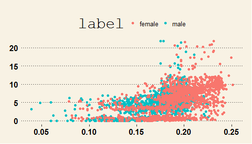
除了使用describe 函数掌握数据的基本状况外,一个必不可少的数据探索步骤,就是使用图形进行探索,我们这里只使用一个例子,帮助大家了解:
### visual exploration of the dataset
voice_Original%>%
  ggplot(aes(x=meanfreq,y=dfrange))+
  geom_point(aes(color=label))+
  theme_wsj()
图形结果如下:
但是我们更关注的是,预测因子之间是不是存在高度的相关性,因为预测因子间的香瓜性对于一些模型,是有不利的影响的。
对于研究预测因子间的相关性,corrplot 包中的corrplot函数提供了很直观的图形方法:
###find correlations between factors
factor_Corr <- cor(voice_Original[,-c(9,21)])
corrplot(factor_Corr,method="number")
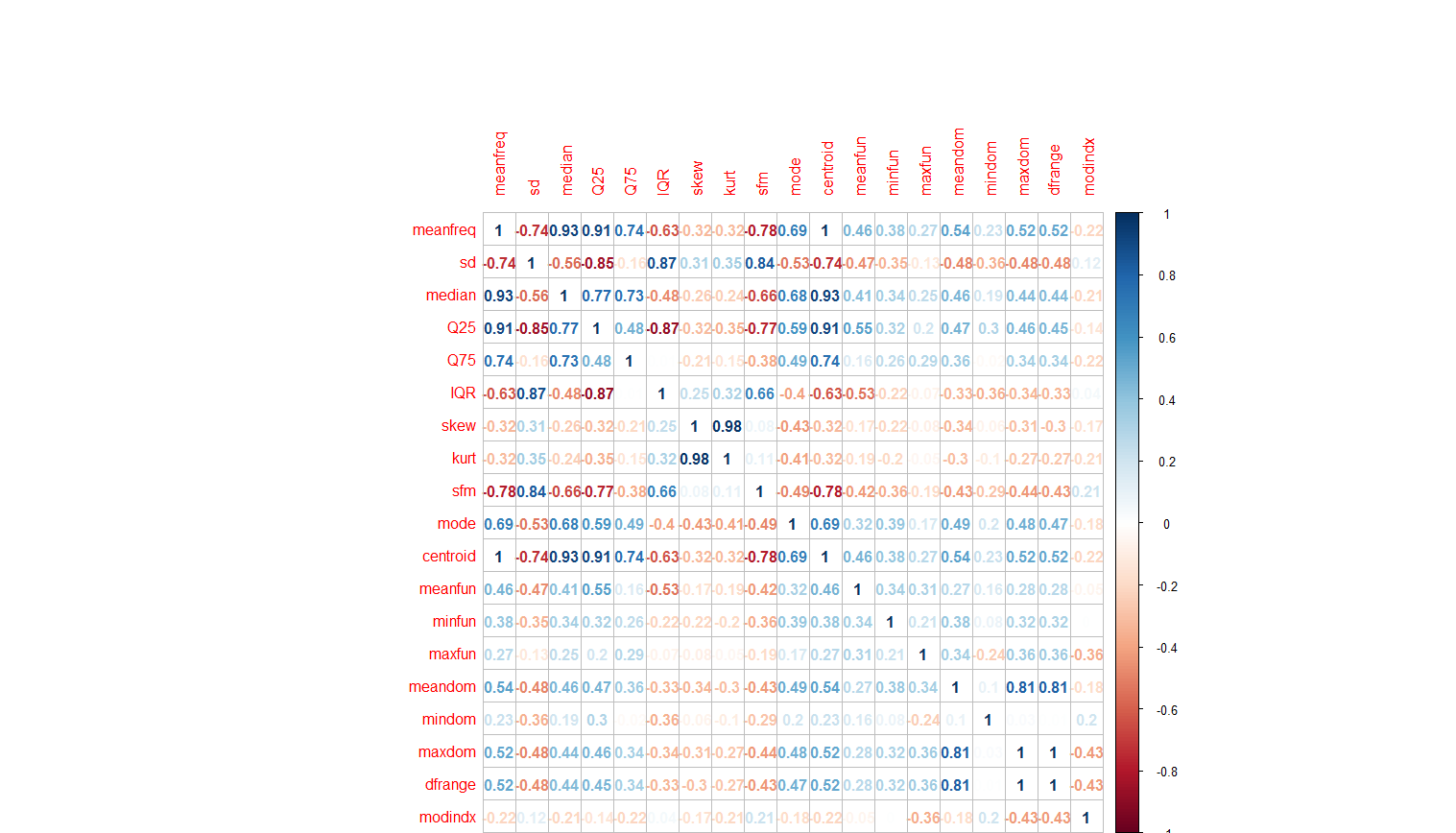
这个相关性矩阵图可以直观地帮助我们发现因子间的强相关性。
步骤3:数据分配与建模
在实际建模过程中,我们不会将所有的数据全部用来进行训练模型,因为相比较模型数据集在训练中的表现,我们更关注模型在训练集,也就是我们的模型没有遇到的数据中的预测表现。
因此,我们将我们的数据集的70%的数据用来训练模型,剩余的30%用来检验模型预测的结果。
sample_Index <- createDataPartition(voice_Original$label,p=0.7,list=FALSE)
voice_Train <- voice_Original[sample_Index,]
voice_Test <- voice_Original[-sample_Index,]
但是我们还没有解决之前我们发现的一些问题,数据的量纲实际上是不一样的,另外某些因子间存在高度的相关性,这对我们的建模是不利的,因此我们需要进行一些预处理,我们又需要用到preProcess 函数:
### preprocess factors for further modeling
pp <- preProcess(voice_Train,method=c("scale","center","pca"))
voice_Train <- predict(pp,voice_Train)
voice_Test <- predict(pp,voice_Test)
我们首先将数值型因子进行了标准化,确保所有的因子在一个量纲上,接着对已经标准化的数据进行主成分分析,消除因子中的高相关性。如果我们看一下我们的现在经过处理的数据,就可以看到:
voice_Train
sp.ent
n missing unique
2218 0 2
label
n missing unique
2218 0 2
PC1
n missing unique Info Mean
2218 0 2216 1 2.084e-17
.05 .10 .25 .50 .75
-5.2623 -3.8212 -2.0470 0.3775 2.0260
.90 .95
3.6648 4.5992
lowest : -9.885 -9.138 -8.560 -8.476 -8.412
PC2
n missing unique Info Mean
2218 0 2216 1 -4.945e-16
.05 .10 .25 .50 .75
-2.7216 -2.0700 -0.8694 0.2569 0.9934
.90 .95
1.5576 2.0555
lowest : -5.528 -5.315 -5.132 -5.103 -5.019
PC3
n missing unique Info Mean
2218 0 2216 1 1.579e-16
.05 .10 .25 .50 .75
-1.6818 -1.3640 -0.7880 -0.2214 0.5731
.90 .95
1.1723 1.6309
lowest : -2.809 -2.536 -2.462 -2.443 -2.407
PC4
n missing unique Info Mean
2218 0 2216 1 -3.583e-16
.05 .10 .25 .50 .75
-1.98986 -1.60536 -0.75468 0.09347 0.86320
.90 .95
1.49494 1.83657
lowest : -7.887 -6.616 -5.735 -5.568 -4.596
PC5
n missing unique Info Mean
2218 0 2216 1 -1.127e-16
.05 .10 .25 .50 .75
-1.8479 -1.2788 -0.5783 0.0941 0.6290
.90 .95
1.1909 1.5739
lowest : -4.595 -3.900 -3.887 -3.787 -3.760
PC6
n missing unique Info Mean
2218 0 2216 1 6.421e-18
.05 .10 .25 .50 .75
-1.56253 -1.03095 -0.39648 0.03999 0.53475
.90 .95
1.10113 1.38224
lowest : -6.971 -6.530 -5.521 -5.510 -5.320
PC7
n missing unique Info Mean
2218 0 2216 1 -2.789e-16
.05 .10 .25 .50 .75
-1.0995 -0.8375 -0.4970 -0.1234 0.4493
.90 .95
1.1055 1.4462
lowest : -3.370 -3.132 -2.977 -2.813 -2.664
PC8
n missing unique Info Mean
2218 0 2216 1 -7.291e-17
.05 .10 .25 .50 .75
-1.18707 -0.96343 -0.51065 -0.02345 0.46939
.90 .95
0.96676 1.28817
lowest : -2.644 -2.611 -2.477 -2.328 -2.261
PC9
n missing unique Info Mean
2218 0 2216 1 4.008e-16
.05 .10 .25 .50 .75
-1.06437 -0.84861 -0.47079 -0.04825 0.42092
.90 .95
0.96161 1.25187
lowest : -2.267 -2.263 -2.095 -2.066 -1.898
PC10
n missing unique Info Mean
2218 0 2216 1 2.387e-16
.05 .10 .25 .50 .75
-0.93065 -0.71784 -0.40541 -0.07025 0.37068
.90 .95
0.82534 1.12412
lowest : -2.160 -1.810 -1.754 -1.744 -1.661
- 1
- 2
- 3
- 4
- 5
- 6
- 7
- 8
- 9
- 10
- 11
- 12
- 13
- 14
- 15
- 16
- 17
- 18
- 19
- 20
- 21
- 22
- 23
- 24
- 25
- 26
- 27
- 28
- 29
- 30
- 31
- 32
- 33
- 34
- 35
- 36
- 37
- 38
- 39
- 40
- 41
- 42
- 43
- 44
- 45
- 46
- 47
- 48
- 49
- 50
- 51
- 52
- 53
- 54
- 55
- 56
- 57
- 58
- 59
- 60
- 61
- 62
- 63
- 64
- 65
- 66
- 67
- 68
- 69
- 70
- 71
- 72
- 73
- 74
- 75
- 76
- 77
- 78
- 79
- 80
- 81
- 82
- 83
- 84
- 85
- 86
- 87
- 88
- 89
- 90
- 91
- 92
- 93
- 94
- 95
- 96
- 97
- 98
- 99
- 100
- 101
- 102
- 103
- 104
- 105
- 106
- 107
- 108
- 109
- 110
- 111
- 112
- 113
- 114
- 115
- 116
- 117
- 118
- 119
- 120
- 121
- 122
- 123
- 124
- 125
- 126
原来的所有数值型因子已经被PC1-PC10取代了。
现在,我们进行一些通用的设置,为不同的模型进行交叉验证比较做好准备。
### define formula
model_Formula <- label~PC1+PC2+PC3+PC4+PC5+PC6+PC7+PC8+PC9+PC10+sp.ent


###set cross-validation parameters

modelControl <- trainControl(method="repeatedcv",number=5,
                             repeats=5,allowParallel=TRUE)
下面我们开始建立我们的第一个模型:逻辑回归模型:
### model 1: logistic regression
glm_Model <- train(model_Formula,
                   data=voice_Train,
                   method="glm",
                   trControl=modelControl)
将模型应用到测试集上,并将结果与真实值进行比较:
voice_Test1 <- voice_Test[,-2]
voice_Test1$glmPrediction <- predict(glm_Model,voice_Test1)
table(voice_Test$label,voice_Test1$glmPrediction)
我们得到的预测结果如下:
         female male
  female    459   16
  male        7  468
我们的逻辑回归你模型将7个女性错判成了男性,16个男性错判成了女性,应该说结果还是不错的。
下面我们再来看看下一个模型:线性判别分析(LDA):
### model 2:linear discrimant analysis
lda_Model <- train(model_Formula,
                   data=voice_Train,
                   method="lda",
                   trControl=modelControl)

voice_Test1$ldaPrediction <- predict(lda_Model,voice_Test1)
table(voice_Test$label,voice_Test1$ldaPrediction)
         female male
  female    454   21
  male        6  469
目前lda方法的预测结果略差于逻辑回归;
第三个模型:随机森林
### model 3: random forrest
rf_Model <- train(model_Formula,
                  data=voice_Train,
                  method="rf",
                  trControl=modelControl,
                  ntrees=500)
voice_Test1$rfPrediction <- predict(rf_Model,voice_Test1)
table(voice_Test$label,voice_Test1$rfPrediction)
         female male
  female    457   18
  male        6  469
可以看到随机森林的结果介于上面两个模型之间。但是模型的结果是存在一定的偶然性的,即因为都使用了交叉验证,每个模型都存在抽样的问题,因此结果之间存在一定的偶然性,所以我们需要对模型进行统计意义上的比较。
但是在此之前,我想提一下并行计算的问题,我们在开始建模之前就使用parallel 和doParallel 两个包设置了并行计算的参数,在modelControl中将allowParallel的值设为了TRUE,就可以帮助我们进行交叉验证时进行并行计算,下面这张图可以帮助我们看到差异:

因为原生的R只支持单进程,通过我们的设置,可以将四个核都使用起来,可以大为减少我们的计算时间。
我们最后的一个步骤就是要将三个模型进行比较,确定我们最优的一个模型:
### which model is the best?
model_Comparison <-
  resamples(list(
    LogisticRegression=glm_Model,
    LinearDiscrimant=lda_Model,
    RandomForest=rf_Model
  ))

summary(model_Comparison)
bwplot(model_Comparison,layout=c(2,1))
下面是我们比较的结果:
Call:
summary.resamples(object = model_Comparison)
Models: LogisticRegression, LinearDiscrimant, RandomForest
Number of resamples: 25
Accuracy
Min. 1st Qu. Median Mean 3rd Qu.
LogisticRegression 0.9572 0.9640 0.9685 0.9699 0.9752
LinearDiscrimant 0.9550 0.9640 0.9662 0.9677 0.9729
RandomForest 0.9505 0.9595 0.9640 0.9641 0.9685
Max. NA
LogisticRegression 0.9819 0
LinearDiscrimant 0.9842 0
RandomForest 0.9774 0
Kappa
Min. 1st Qu. Median Mean 3rd Qu.
LogisticRegression 0.9144 0.9279 0.9369 0.9398 0.9505
LinearDiscrimant 0.9099 0.9279 0.9324 0.9354 0.9457
RandomForest 0.9009 0.9189 0.9279 0.9282 0.9369
Max. NA
LogisticRegression 0.9639 0
LinearDiscrimant 0.9685 0
RandomForest 0.9549 0
- 1
- 2
- 3
- 4
- 5
- 6
- 7
- 8
- 9
- 10
- 11
- 12
- 13
- 14
- 15
- 16
- 17
- 18
- 19
- 20
- 21
- 22
- 23
- 24
- 25
- 1
- 2
- 3
- 4
- 5
- 6
- 7
- 8
- 9
- 10
- 11
- 12
- 13
- 14
- 15
- 16
- 17
- 18
- 19
- 20
- 21
- 22
- 23
- 24
- 25
结果从准确率和Kappa值两个方面对数据进行了比较,可以帮助我们了解模型的实际表现,当然我们也可以通过图形展现预测结果:
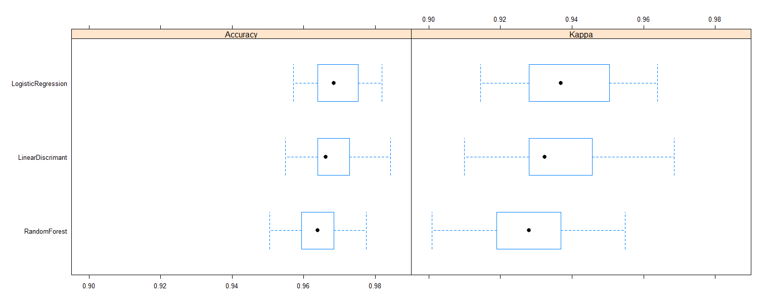
根据结果,我们可以看到,其实逻辑回归的结果还是比较好的。
所以我们可以将逻辑回归的结果作为我们最终使用的模型。


 839
839

 被折叠的 条评论
为什么被折叠?
被折叠的 条评论
为什么被折叠?
 到【灌水乐园】发言


