


本文只是记录一下实现的代码,具体的思想还请看cs231n的课程笔记,其讲解的非常好,智能单元翻译的也很不错。
一、CIFAR-10数据集:
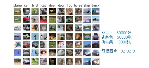
图1 CIFAR-10示例
二、KNN
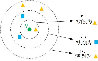
图2 KNN分类器示例
如图所示,K的取值不同得出来的分类结果也可能是不同的,因此需要对k进行寻参,找出在训练机上最好的k,来进行测试。
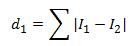
求两幅图片的相似性,KNN使用的是距离度量,但是距离定义方式也有很多种,比如L1距离、L2距离。
1、L1距离:
其中 和
和 表示两幅图片对应的向量,一般对图像进行计算的时候,都是把一幅图片拉成一行或者是一列, 如下图(没有对图片拉成向量):
和表示两幅图片对应的向量,一般对图像进行计算的时候,都是把一幅图片拉成一行或者是一列, 如下图(没有对图片拉成向量):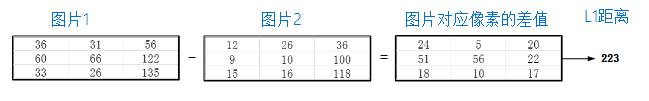
图3 L1距离
2、L2距离:
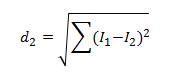
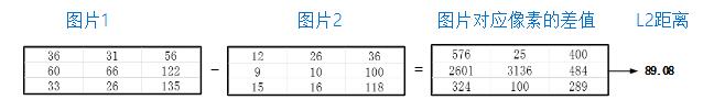
图4 L2距离
本文采用L2距离来计算两个图片之间的距离。KNN思想比较简单,到这里就可以实现了。
1> 首先读取数据集:
# -*- coding: utf-8 -*-
"""
Created on Sun May  7 19:32:30 2017

@author: admin
"""
import numpy as np
import pickle
import os

def Load_CIFAR_Batch(filename):
    with open(filename, 'rb') as f:
        datadict = pickle.load(f, encoding = 'latin1')
        X = datadict['data']
        Y = datadict['labels']
        X = X.reshape(10000, 3, 32, 32).transpose(0, 2, 3, 1).astype('float')#1000*32*32*3
        Y = np.array(Y)
        return X, Y

def Load_CIFAR10(Root):
    xs = []
    ys = []

    for b in range(1,  6):
        f = os.path.join(Root, 'data_batch_%d'%(b, ))
        X, Y = Load_CIFAR_Batch(f)
        xs.append(X)
        ys.append(Y)
    Xtr = np.concatenate(xs)
    Ytr = np.concatenate(ys)

    del X, Y
    Xte, Yte = Load_CIFAR_Batch(os.path.join(Root, 'test_batch'))
return Xtr, Ytr, Xte, Ytedef Load_CIFAR10(Root):
# -*- coding: utf-8 -*-
"""
Created on Thu May  4 20:27:04 2017

@author: admin
"""

import numpy as np

from LoadData import Load_CIFAR10


class KNN(object):
    def __init__(self):
        pass
    def train(self, X, Y):
        self.X_train = X
        self.Y_train = Y
    def predict(self, X, k=1):
        dist_matrix = self.compute_L2_distance(X)
        return self.predict_labels(dist_matrix, k = k)

    def compute_L2_distance(self, X):
        num_test = X.shape[0]
        num_train = self.X_train.shape[0]
        dist_matrix = np.zeros((num_test, num_train))
        for i in range(num_test):#求出第i个测试样本与所有样本的距离,(X[i, :] - self.X_train)是测试样本第i行减去训练样本的全部行
            square_distance = np.sum((X[i, :] - self.X_train)*(X[i, :] - self.X_train), axis = 1)
            dist_matrix[i, :] = np.sqrt(square_distance)
        return dist_matrix

    def predict_labels(self, dist_matrix, k = 1):
        num_test = dist_matrix.shape[0]
        y_predict = np.zeros(num_test)
        for i in range(num_test):
            nearest_y = []
            argsort_distance = np.argsort(dist_matrix[i, :])
            nearest_y = argsort_distance[0:k]
            nearest_labels = list(self.Y_train[nearest_y])
            most_common_label = max(set(nearest_labels), key = nearest_labels.count)

            for num in set(nearest_labels):
                if nearest_labels.count(num) == nearest_labels.count(most_common_label):
                    if num < most_common_label:
                        most_common_label = num
            y_predict[i] = most_common_label


        return y_predict

Xtr, Ytr, Xte, Yte = Load_CIFAR10('cifar-10-batches-py')
Xtr_rows = Xtr.reshape(Xtr.shape[0], 32*32*3)
Xte_rows = Xte.reshape(Xte.shape[0], 32*32*3)

nn = KNN()
print ("trainning........")
nn.train(Xtr_rows, Ytr)
print ("trainning over!")
print ("predicting........")
Yte_predict = nn.predict(Xte_rows)
print ("predicted!")
print ('accuracy: %f' % (np.mean(Yte_predict == Yte)))KNN分类器的缺点:
1、分类器必须要存储所有的训练数据,以便测试数据用来计算距离,因此当数据集很大时,需要很大的存储空间。
2、对于每一张测试图像,它都需要和所有的训练图像进行比较,因此它是比较耗时的。
二、多类SVM
线性分类器:一幅图像经过一个线性映射,得到各分类类别的得分,得分的高低代表图像属于该类别的可能性的高低。
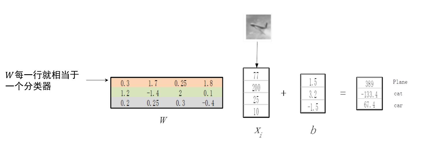
图5 线性分类器
多类SVM损失函数采用Hinge Loss,如下,这个很奇妙,这个delta具体的物理意义是什么,加入正则项SVM就有了最大间隔的意义,这个是好理解的,但是损失中的delta的物理意义,还需要仔细思考一下。

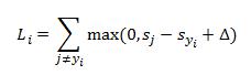
例如:有3个分类,并且得到的分值为

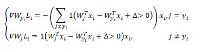
为使得损失函数最小化,采用梯度下降法,在求每个样本损失的时候,同时计算梯度。
二、Softmax分类器
(NND好不容易弄完,可恶的CSDN提交的时候,居然把往后的部分弄没了!)因为SVM和Softmax 同属于线性分类器,对于线性训练部分是一样的,SVM和Softmax在对分类结果的表达上是不同的。还是先介绍Softmax: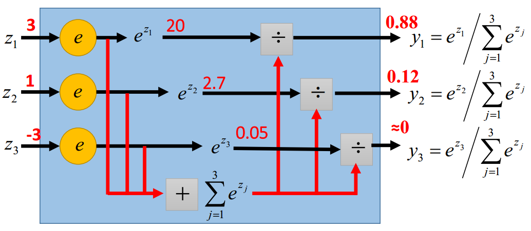
图6 Softmax示例
从上图可以看出Softmax对于计算出的值,进行归一化,转化成概率的形式,这样对于每一种类别的选择,有一定的把握性,对于分类结果也有很好的解释性。而SVM最终选择的类别只是得分最高的,但是这个分值,却不能给予一个直观的解释。
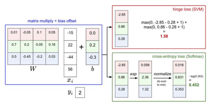
图7 SVM和Softmax对比
从图中可以看到SVM和Softmax前半部分的计算方式一样的,只是对后面的损失计算和对分结果的处理方式是不一样的。
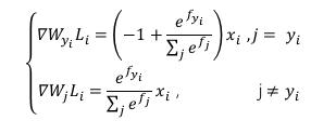
softmax的损失函数是交叉熵损失,那么第i个样本的损失形式如下:
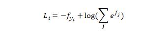
这里给出的Softmax损失函数,只是很精简的部分,里面有很多的理论推导,这里都省略了,需要了解的自行参考其他文献。为使得损失函数最小化,同样采用梯度下降法。
Softmax损失计算实现:
# -*- coding: utf-8 -*-
"""
Created on Sun May  7 14:21:49 2017

@author: admin
"""

import numpy as np

def Softmax_Loss(W, X, Y, reg):
    dW = np.zeros_like(W)#W's shape (C, D)
    num_classes = W.shape[0]
    num_train = X.shape[1]#X's shape (D, N)
    loss_value = 0.0

    for i in range(num_train):
        scores = W.dot(X[:, i])
        shift_scores = scores - max(scores)
        loss_i = -shift_scores[Y[i]] + np.log(sum(np.exp(shift_scores)))
        loss_value += loss_i
        for j in range(num_classes):
            softmax_output = np.exp(shift_scores[j])/sum(np.exp(shift_scores))
            if j == Y[i]:
                dW[j, :] = dW[j, :] - X[:, i] + softmax_output * X[:, i]
            else:
                dW[j, :] = dW[j, :] + softmax_output * X[:, i]

    loss_value /= num_train
    loss_value += 0.5 * reg * np.sum(W * W)
    dW = dW/num_train + reg * W

    return loss_value, dW
# -*- coding: utf-8 -*-
"""
Created on Sun May  7 15:42:42 2017

@author: admin
"""

import numpy as np


from SVM_Loss import SVM_Loss
from Softmax_Loss import Softmax_Loss


class Linear_Classifier:
    def __init__(self):
        self.W = None

    def train(self, X, Y, learning_rate = 1e-3, reg = 1e-5, num_iters = 100,
              batch_size = 200, verbose = False):
        """
        输入
        X: 形状为(D, N)的numpy数组,包含N个训练样本, 每个训练样本的维数是D
        Y:形状为(N,)的numpy数组,包含N个训练样本的标签,其中Y[i] = c,表示
        样本X[i]对应的标签为c,且满足0 <= c < C,C为总共有C个类别
        learning_rate:学习率,最优化时的步长
        reg:正则向对应lambda的值
        num_iters:最优化过程中的迭代次数
        batch_size:每一步训练样本的个数
        verbos:如果为真,打印在优化时的过程

        输出:
        一个列表,其包含每次训练迭代损失函数的值。
        """
        dim, num_train = X.shape
        num_classes = np.max(Y)+1
        if self.W is None:
            self.W = 0.001 * np.random.randn(num_classes, dim)
        loss_history = []
        for it in range(num_iters):
#            print("The number iters: %d" % (it))
            X_batch = None
            Y_batch = None
            """
            从训练数据集中抽取batch_size个元素及其对应的标签,用于此轮的梯度下降。
            将数据存放于X_batch中,并将其对应的标签存放于Y_batch中,采样后X_batch
            的形状为(dim, bat_size),Y_batch的形状为(batch_size,)
            提示:
            使用np.random.choice生成的是索引,替换采样速度快于不替换采样的速度。
            """
#            idx = np.random.choice(num_train, batch_size, replace = False)
#            X_batch = X[idx]
#            Y_batch = Y[idx]
            rand_idx = np.random.choice(num_train, batch_size)
            X_batch = X[:, rand_idx]
            Y_batch = Y[rand_idx]
            #计算损失和梯度
            loss, gradient = self.loss(X_batch, Y_batch, reg)
            loss_history.append(loss)

            self.W = self.W - learning_rate * gradient

            if verbose and it % 100 == 0:
                print('iteration %d / %d: loss %f' % (it, num_iters, loss))

        return loss_history

    def Predict(self, X):
        """
        #X (D, N)
        """
        y_pred = np.zeros(X.shape[1])
        #scores = X.dot(self.W) #(N, C)]
        scores = np.dot(self.W, X)
        y_pred = np.argmax(scores, axis = 0)

        return y_pred

    def loss(self, X_batch, Y_batch, reg):
        pass


class Linear_SVM(Linear_Classifier):
    def loss(self, X_batch, Y_batch, reg):
        return SVM_Loss(self.W,  X_batch, Y_batch, reg)

class Softmax(Linear_Classifier):
    def loss(self, X_batch, Y_batch, reg):
        return Softmax_Loss(self.W,  X_batch, Y_batch, reg)
SVM分类器:
# -*- coding: utf-8 -*-
"""
Created on Sun May  7 19:38:27 2017

@author: admin
"""

import numpy as np
from SVM_Loss import SVM_Loss
from LoadData import Load_CIFAR10
import matplotlib.pyplot as plt
from Linear_Classifier import Linear_SVM
import time

Xtr, Ytr, Xte, Yte = Load_CIFAR10('cifar-10-batches-py')

print ('Training data shape: ', Xtr.shape)
print ('Training labels shape: ', Ytr.shape)
print ('Test data shape: ', Xte.shape)
print ('Test labels shape: ', Yte.shape)

#显示数据集样式
'''
classes = ['plane', 'car', 'bird', 'cat', 'deer', 'dog', 'frog', 'horse', 'ship', 'truck']
num_classes = len(classes)
samples_per_class = 10

for y, cls in enumerate(classes):
    idxs = np.flatnonzero(Ytr == y)#Return the indices of the non-zero elements of the input array
    idxs = np.random.choice(idxs, samples_per_class, replace=False)
    for i, idx in enumerate(idxs):
        plt_idx = i * num_classes + y + 1
        plt.subplot(samples_per_class, num_classes, plt_idx)
        plt.imshow(Xtr[idx].astype('uint8'))
        plt.axis('off')
        if i == 0:
            plt.title(cls)
plt.show()
'''

#添加验证集
num_training = 49000
num_validation = 1000
num_test = 1000

# Our validation set will be num_validation points from the original
# training set.
mask = range(num_training, num_training + num_validation)
X_val = Xtr[mask]
y_val = Ytr[mask]

# Our training set will be the first num_train points from the original
# training set.
mask = range(num_training)
X_train = Xtr[mask]
y_train = Ytr[mask]

# We use the first num_test points of the original test set as our
# test set.
mask = range(num_test)
X_test = Xte[mask]
y_test = Yte[mask]

print ('Train data shape: ', X_train.shape)
print ('Train labels shape: ', y_train.shape)
print ('Validation data shape: ', X_val.shape)
print ('Validation labels shape: ', y_val.shape)
print ('Test data shape: ', X_test.shape)
print ('Test labels shape: ', y_test.shape)


#把图片展成一行
X_train = np.reshape(X_train, (X_train.shape[0], -1))
X_val = np.reshape(X_val, (X_val.shape[0], -1))
X_test = np.reshape(X_test, (X_test.shape[0], -1))

# 检查数据集的形状
print ('Training data shape: ', X_train.shape)
print ('Validation data shape: ', X_val.shape)
print ('Test data shape: ', X_test.shape)

#预处理
#1、得出训练集中图片的均值,按列求均值
mean_image = np.mean(X_train, axis=0)
print (mean_image[:10]) # 打印前10个元素
plt.figure(figsize=(4,4))
plt.imshow(mean_image.reshape((32,32,3)).astype('uint8')) # 可视化均值图片

#2、让训练集和测试集都减去均值图片
X_train -= mean_image
X_val -= mean_image
X_test -= mean_image

#3、对每幅图片添加一个维度,也就是生产一个N*1维度的数组,然后水平拼接
#然后对训练和测试集进行转置,换成D*N的形式
print("Preprocessing........")
X_train = np.hstack([X_train, np.ones((X_train.shape[0], 1))]).T
X_val = np.hstack([X_val, np.ones((X_val.shape[0], 1))]).T
X_test = np.hstack([X_test, np.ones((X_test.shape[0], 1))]).T
print ('Training data shape: ', X_train.shape)
print ('Validation data shape: ', X_val.shape)
print ('Test data shape: ', X_test.shape)
print("Preprocessed!!!")

"""
SVM Classifier
"""

#W = np.random.randn(3073, 10)*0.0001
#loss, gradient = SVM_Loss(W, X_train, y_train, 0.00001)
#print ("loss: %f" % (loss,))

'''
tic = time.time()
svm = Linear_SVM()
print ("Training........")
loss_history = svm.train(X_train, y_train, learning_rate = 1e-7, reg = 5e4,
                      num_iters = 1500, verbose = True)
print ("Training Over!")
toc = time.time()

print ("That took %fs" % (toc - tic))

plt.plot(loss_history)
plt.xlabel("Iteration number")
plt.ylabel("Loss value")


#在训练集和测试集上面的正确率
y_train_pred = svm.Predict(X_train)
print ('training accuracy: %f' % (np.mean(y_train == y_train_pred), ))
y_val_pred = svm.Predict(X_val)
print ('validation accuracy: %f' % (np.mean(y_val == y_val_pred), ))

'''

learning_rates = [1e-7, 2e-7, 5e-7, 1e-6]
regularization_strengths = [1e4, 2e4, 5e4, 1e5, 5e5, 1e6]

# results is dictionary mapping tuples of the form
#寻参
results = {}
best_val = -1   # The highest validation accuracy that we have seen so far.
best_svm = None # The LinearSVM object that achieved the highest validation rate.


for learning in learning_rates:
    for regularization in regularization_strengths:
        svm = Linear_SVM()
        svm.train(X_train, y_train, learning_rate=learning, reg=regularization,
                              num_iters=200)
        y_train_pred = svm.Predict(X_train)
        train_accuracy = np.mean(y_train == y_train_pred)
        print ('training accuracy: %f' % (train_accuracy))
        y_val_pred = svm.Predict(X_val)
        val_accuracy = np.mean(y_val == y_val_pred)
        print ('validation accuracy: %f' % (val_accuracy))

        if val_accuracy > best_val:
            best_val = val_accuracy
            best_svm = svm

        results[(learning, regularization)] = (train_accuracy, val_accuracy)

y_test_pred = best_svm.Predict(X_test)
test_accuracy = np.mean(y_test == y_test_pred)
print ('linear SVM on raw pixels final test set accuracy: %f' % test_accuracy)


# Visualize the learned weights for each class.
# Depending on your choice of learning rate and regularization strength, these may
# or may not be nice to look at.
w = best_svm.W[:,:-1] # strip out the bias
w = w.reshape(10, 32, 32, 3)
w_min, w_max = np.min(w), np.max(w)
classes = ['plane', 'car', 'bird', 'cat', 'deer', 'dog', 'frog', 'horse', 'ship', 'truck']
for i in range(10):
  plt.subplot(2, 5, i + 1)

  # Rescale the weights to be between 0 and 255
  wimg = 255.0 * (w[i].squeeze() - w_min) / (w_max - w_min)
  plt.imshow(wimg.astype('uint8'))
  plt.axis('off')
  plt.title(classes[i])
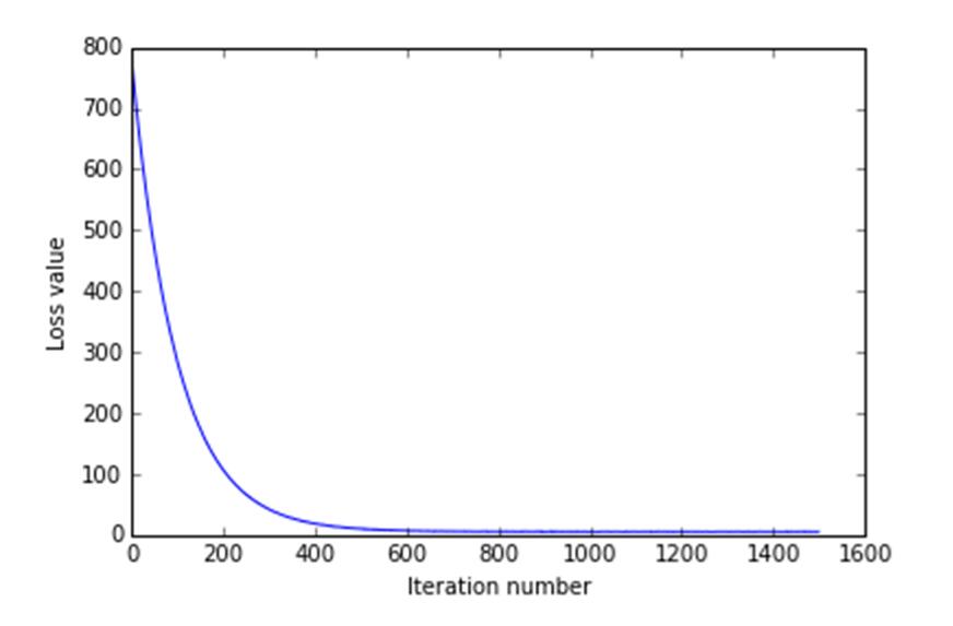
图8 迭代过程中的损失值
由于学习速率和正则向的不同,对损失函数的收敛速度和分类结果的正确率有很大的影响,本此实验进行了24轮寻参,在验证集上的正确率,如下:
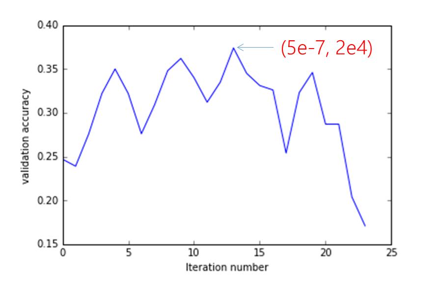
图9 寻参过程中验证集的正确率
SVM学习的最优权重,显示化如下:
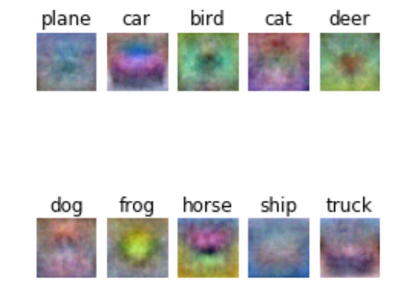
图10 SVM最优权重
SVM在测试集上的正确率为36.5%
Softmax分类器实现:
# -*- coding: utf-8 -*-
"""
Created on Mon May  8 14:43:25 2017

@author: admin
"""

import numpy as np
from Softmax_Loss import Softmax_Loss
from LoadData import Load_CIFAR10
import matplotlib.pyplot as plt
from Linear_Classifier import Softmax


Xtr, Ytr, Xte, Yte = Load_CIFAR10('cifar-10-batches-py')

print ('Training data shape: ', Xtr.shape)
print ('Training labels shape: ', Ytr.shape)
print ('Test data shape: ', Xte.shape)
print ('Test labels shape: ', Yte.shape)

#添加验证集
num_training = 49000
num_validation = 1000
num_test = 1000

# Our validation set will be num_validation points from the original
# training set.
mask = range(num_training, num_training + num_validation)
X_val = Xtr[mask]
y_val = Ytr[mask]

# Our training set will be the first num_train points from the original
# training set.
mask = range(num_training)
X_train = Xtr[mask]
y_train = Ytr[mask]

# We use the first num_test points of the original test set as our
# test set.
mask = range(num_test)
X_test = Xte[mask]
y_test = Yte[mask]

#把图片展成一行
X_train = np.reshape(X_train, (X_train.shape[0], -1))
X_val = np.reshape(X_val, (X_val.shape[0], -1))
X_test = np.reshape(X_test, (X_test.shape[0], -1))

# 检查数据集的形状
print ('Training data shape: ', X_train.shape)
print ('Validation data shape: ', X_val.shape)
print ('Test data shape: ', X_test.shape)

#预处理
#1、得出训练集中图片的均值,按列求均值
mean_image = np.mean(X_train, axis=0)
print (mean_image[:10]) # 打印前10个元素
plt.figure(figsize=(4,4))
plt.imshow(mean_image.reshape((32,32,3)).astype('uint8')) # 可视化均值图片

#2、让训练集和测试集都减去均值图片
X_train -= mean_image
X_val -= mean_image
X_test -= mean_image

#3、对每幅图片添加一个维度,也就是生产一个N*1维度的数组,然后水平拼接
#然后对训练和测试集进行转置,换成D*N的形式
print("Preprocessing........")
X_train = np.hstack([X_train, np.ones((X_train.shape[0], 1))]).T
X_val = np.hstack([X_val, np.ones((X_val.shape[0], 1))]).T
X_test = np.hstack([X_test, np.ones((X_test.shape[0], 1))]).T
print ('Training data shape: ', X_train.shape)
print ('Validation data shape: ', X_val.shape)
print ('Test data shape: ', X_test.shape)
print("Preprocessed!!!")

results = {}
best_val = -1
best_softmax = None
learning_rates = [5e-6, 1e-7, 5e-7]
regularization_strengths = [1e4, 5e4, 1e5]
params = [(x,y) for x in learning_rates for y in regularization_strengths ]
for lrate, regular in params:
    softmax = Softmax()
    loss_hist = softmax.train(X_train, y_train, learning_rate=lrate, reg=regular,
                             num_iters=700, verbose=True)
    y_train_pred = softmax.Predict(X_train)
    accuracy_train = np.mean( y_train == y_train_pred)
    y_val_pred = softmax.Predict(X_val)
    accuracy_val = np.mean(y_val == y_val_pred)
    results[(lrate, regular)] = (accuracy_train, accuracy_val)
    if(best_val < accuracy_val):
        best_val = accuracy_val
        best_softmax = softmax

# Print out results.
for lr, reg in sorted(results):
    train_accuracy, val_accuracy = results[(lr, reg)]
    print ('lr %e reg %e train accuracy: %f val accuracy: %f' % (
                lr, reg, train_accuracy, val_accuracy))

print ('best validation accuracy achieved during cross-validation: %f' % best_val)

y_test_pred = best_softmax.Predict(X_test)
test_accuracy = np.mean(y_test == y_test_pred)
print ('linear Softmax on raw pixels final test set accuracy: %f' % test_accuracy)

w = best_softmax.W[:,:-1] # strip out the bias
w = w.reshape(10, 32, 32, 3)
w_min, w_max = np.min(w), np.max(w)
classes = ['plane', 'car', 'bird', 'cat', 'deer', 'dog', 'frog', 'horse', 'ship', 'truck']
for i in range(10):
  plt.subplot(2, 5, i + 1)

  # Rescale the weights to be between 0 and 255
  wimg = 255.0 * (w[i].squeeze() - w_min) / (w_max - w_min)
  plt.imshow(wimg.astype('uint8'))
  plt.axis('off')
  plt.title(classes[i])
Softmax经过9次寻参,对应验证集的正确率如下所示:
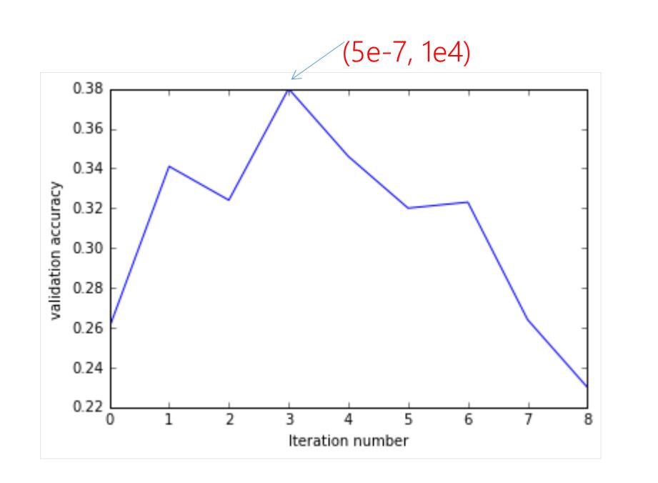
图11 寻参过程中验证集正确率
Softmax学到的最优权重:
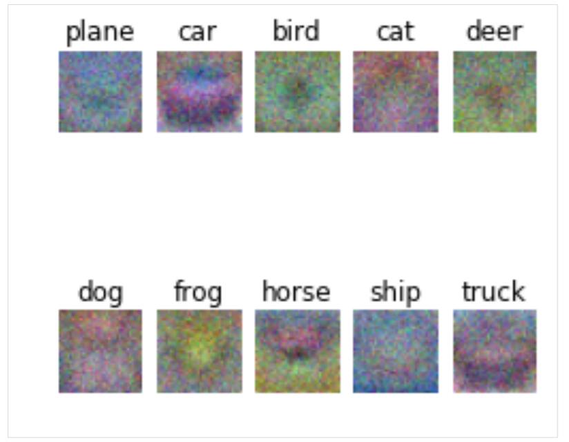
图12 最优权重
从权重显示上来看,他们学习的分类几乎差不多,因此从这里也可以推断,他们两个在CIFAR10上的正确率应该也差不多。
在经过寻参和优化权重之后,Softmax在测试集上的正确率为36.9%。其实跟SVM差不多。
SVM和Softmax总结:
1、从运行结果来看,Softmax和SVM的表现相当。
2、对于SVM来说只要满足边界值,就停止计算损失,但是对于Softmax分类器来说,它会一直要求正确分类的可能性尽可能的高。


 4388
4388

 被折叠的 条评论
为什么被折叠?
被折叠的 条评论
为什么被折叠?
 到【灌水乐园】发言


