计算两个文档的相似度

出处“我爱自然语言处理”：www.52nlp.cn

前几天，我发布了一个和在线教育相关的网站：课程图谱，这个网站的目的通过对公开课的导航、推荐和点评等功能方便大家找到感兴趣的公开课，特别是目前最火的Coursera，Udacity等公开课平台上的课程。在发布之前，遇到的一个问题是如何找到两个相关的公开课，最早的计划是通过用户对课程的关注和用户对用户的关注来做推荐，譬如“你关注的朋友也关注这些课程”，但是问题是网站发布之前，我还没有积累用户关注的数据。另外一个想法是提前给课程打好标签，通过标签来计算它门之间的相似度，不过这是一个人工标注的过程，需要一定的时间。当然，另一个很自然的想法是通过课程的文本内容来计算课程之间的相似度，公开课相对来说有很多的文本描述信息，从文本分析的角度来处理这种推荐系统的冷启动问题应该不失为一个好的处理方法。通过一些调研和之前的一些工作经验，最终考虑采用Topic model来解决这个问题，其实方案很简单，就是将两个公开课的文本内容映射到topic的维度，然后再计算其相似度。然后的然后就通过google发现了gensim这个强大的Python工具包，它的简介只有一句话：topic modelling for humans, 用过之后，只能由衷的说一句：感谢上帝，感谢Google，感谢开源！

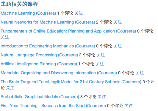
当前课程图谱中所有课程之间的相似度全部基于gensim计算，自己写的调用代码不到一百行，topic模型采用LSI(Latent semantic indexing, 中文译为浅层语义索引），LSI和LSA（Latent semantic analysis，中文译为浅层语义分析）这两个名词常常混在一起，事实上，在维基百科上，有建议将这两个名词合二为一。以下是课程图谱的一个效果图，课程为著名的机器学习专家Andrew Ng教授在Coursera的机器学习公开课，图片显示的是主题模型计算后排名前10的相关课程，Andrew Ng教授同时也是Coursera的创始人之一：

　　　　　

最后回到这篇文章的主题，我将会分3个部分介绍，首先介绍一些相关知识点，不过不会详细介绍每个知识点的细节，主要是简要的描述一下同时提供一些互联网上现有的不错的参考资料，如果读者已经很熟悉，可以直接跳过去；第二部分我会介绍gensim的安装和使用，特别是如何计算课程图谱上课程之间的相似度的；第三部分包括如何基于全量的英文维基百科（400多万文章，压缩后9个多G的语料）在一个4g内存的macbook上训练LSI模型和LDA模型，以及如何将其应用到课程图谱上来改进课程之前的相似度的效果，注意课程图谱的课程内容主要是英文，目前的效果还是第二部分的结果，第三部分我们一起来实现。如果你的英文没问题，第二，第三部分可以直接阅读gensim的tutorail，我所做的事情主要是基于这个tutorail在课程图谱上做了一些验证。

一、相关的知识点及参考资料

这篇文章不会写很长，但是涉及的知识点蛮多，所以首先会在这里介绍相关的知识点，了解的同学可以一笑而过，不了解的同学最好能做一些预习，这对于你了解topic model以及gensim更有好处。如果以后时间允许，我可能会基于其中的某几个点写一篇比较详细的介绍性的文章。不过任何知识点首推维基百科，然后才是下面我所罗列的参考资料。

1） TF-IDF，余弦相似度，向量空间模型
这几个知识点在信息检索中是最基本的，入门级的参考资料可以看看吴军老师在《数学之美》中第11章“如何确定网页和查询的相关性”和第14章“余弦定理和新闻的分类”中的通俗介绍或者阮一峰老师写的两篇科普文章“TF-IDF与余弦相似性的应用（一）：自动提取关键词”和“TF-IDF与余弦相似性的应用（二）：找出相似文章”。

专业一点的参考资料推荐王斌老师在中科院所授的研究生课程“现代信息检索(Modern Information Retrieval)”的课件，其中“第六讲向量模型及权重计算”和该主题相关。或者更详细的可参考王斌老师翻译的经典的《信息检索导论》第6章或者其它相关的信息检索书籍。

2）SVD和LSI
想了解LSI一定要知道SVD（Singular value decomposition, 中文译为奇异值分解），而SVD的作用不仅仅局限于LSI，在很多地方都能见到其身影，SVD自诞生之后，其应用领域不断被发掘，可以不夸张的说如果学了线性代数而不明白SVD，基本上等于没学。想快速了解或复习SVD的同学可以参考这个英文tutorail: Singular Value Decomposition Tutorial , 当然更推荐MIT教授Gilbert Strang的线性代数公开课和相关书籍，你可以直接在网易公开课看相关章节的视频。

关于LSI，简单说两句，一种情况下我们考察两个词的关系常常考虑的是它们在一个窗口长度（譬如一句话，一段话或一个文章）里的共现情况，在语料库语言学里有个专业点叫法叫Collocation，中文译为搭配或词语搭配。而LSI所做的是挖掘如下这层词语关系：A和C共现，B和C共现，目标是找到A和B的隐含关系，学术一点的叫法是second-order co-ocurrence。以下引用百度空间上一篇介绍相关参考资料时的简要描述：

LSI本质上识别了以文档为单位的second-order co-ocurrence的单词并归入同一个子空间。因此：
1）落在同一子空间的单词不一定是同义词，甚至不一定是在同情景下出现的单词，对于长篇文档尤其如是。
2）LSI根本无法处理一词多义的单词（多义词），多义词会导致LSI效果变差。

A persistent myth in search marketing circles is that LSI grants contextuality; i.e., terms occurring in the same context. This is not always the case. Consider two documents X and Y and three terms A, B and C and wherein:

A and B do not co-occur.
X mentions terms A and C
Y mentions terms B and C.

:. A—C—B

The common denominator is C, so we define this relation as an in-transit co-occurrence since both A and B occur while in transit with C. This is called second-order co-occurrence and is a special case of high-order co-occurrence.

其实我也推荐国外这篇由Dr. E. Garcia所写的SVD与LSI的通俗教程，这个系列最早是微博上有朋友推荐，不过发现英文原始网站上内容已经被其主人下架了，原因不得而知。幸好还有Google,在CSDN上我找到了这个系列“SVD与LSI教程系列”，不过很可惜很多图片都看不见了，如果哪位同学发现更好的版本或有原始的完整版本，可以告诉我，不甚感激！

不过幸好原文作者写了两个简要的PDF Tutorail版本：

Singular Value Decomposition (SVD)- A Fast Track Tutorial

Latent Semantic Indexing (LSI) A Fast Track Tutorial

这两个简明版本主要是通过简单的例子直观告诉你什么是SVD，什么是LSI，非常不错。

这几个版本的pdf文件我在微盘上上传了一个打包文件，也可以从这里下载：svd-lsi-doc.tar.gz

3) LDA
这个啥也不说了，隆重推荐我曾经在腾讯工作时的leader rickjin的”LDA数学八卦“系列，通俗易懂，娓娓道来，另外rick的其他系列也是非常值得一读的。

二、gensim的安装和使用

1、安装
gensim依赖NumPy和SciPy这两大Python科学计算工具包，一种简单的安装方法是pip install，但是国内因为网络的缘故常常失败。所以我是下载了gensim的源代码包安装的。gensim的这个官方安装页面很详细的列举了兼容的Python和NumPy, SciPy的版本号以及安装步骤，感兴趣的同学可以直接参考。下面我仅仅说明在Ubuntu和Mac OS下的安装：

1）我的VPS是64位的Ubuntu 12.04，所以安装numpy和scipy比较简单”sudo apt-get install python-numpy python-scipy”, 之后解压gensim的安装包，直接“sudo python setup.py install”即可；

2）我的本是macbook pro，在mac os上安装numpy和scipy的源码包废了一下周折，特别是后者，一直提示fortran相关的东西没有，google了一下，发现很多人在mac上安装scipy的时候都遇到了这个问题，最后通过homebrew安装了gfortran才搞定：“brew install gfortran”,之后仍然是“sudo python setpy.py install” numpy 和 scipy即可；

2、使用
gensim的官方tutorial非常详细，英文ok的同学可以直接参考。以下我会按自己的理解举一个例子说明如何使用gensim，这个例子不同于gensim官方的例子，可以作为一个补充。上一节提到了一个文档：Latent Semantic Indexing (LSI) A Fast Track Tutorial , 这个例子的来源就是这个文档所举的3个一句话doc。首先让我们在命令行中打开python，做一些准备工作:

>>> from gensim import corpora, models, similarities
>>> import logging
>>> logging.basicConfig(format=’%(asctime)s : %(levelname)s : %(message)s’, level=logging.INFO)

然后将上面那个文档中的例子作为文档输入，在Python中用document list表示：

>>> documents = [“Shipment of gold damaged in a fire”,
… “Delivery of silver arrived in a silver truck”,
… “Shipment of gold arrived in a truck”]

正常情况下，需要对英文文本做一些预处理工作，譬如去停用词，对文本进行tokenize，stemming以及过滤掉低频的词，但是为了说明问题，也是为了和这篇”LSI Fast Track Tutorial”保持一致，以下的预处理仅仅是将英文单词小写化：

>>> texts = [[word for word in document.lower().split()] for document in documents]
>>> print texts
[[‘shipment’, ‘of’, ‘gold’, ‘damaged’, ‘in’, ‘a’, ‘fire’], [‘delivery’, ‘of’, ‘silver’, ‘arrived’, ‘in’, ‘a’, ‘silver’, ‘truck’], [‘shipment’, ‘of’, ‘gold’, ‘arrived’, ‘in’, ‘a’, ‘truck’]]

我们可以通过这些文档抽取一个“词袋（bag-of-words)“，将文档的token映射为id：

>>> dictionary = corpora.Dictionary(texts)
>>> print dictionary
Dictionary(11 unique tokens)
>>> print dictionary.token2id
{‘a': 0, ‘damaged': 1, ‘gold': 3, ‘fire': 2, ‘of': 5, ‘delivery': 8, ‘arrived': 7, ‘shipment': 6, ‘in': 4, ‘truck': 10, ‘silver': 9}

然后就可以将用字符串表示的文档转换为用id表示的文档向量：

>>> corpus = [dictionary.doc2bow(text) for text in texts]
>>> print corpus
[[(0, 1), (1, 1), (2, 1), (3, 1), (4, 1), (5, 1), (6, 1)], [(0, 1), (4, 1), (5, 1), (7, 1), (8, 1), (9, 2), (10, 1)], [(0, 1), (3, 1), (4, 1), (5, 1), (6, 1), (7, 1), (10, 1)]]

例如（9，2）这个元素代表第二篇文档中id为9的单词“silver”出现了2次。

有了这些信息，我们就可以基于这些“训练文档”计算一个TF-IDF“模型”：

>>> tfidf = models.TfidfModel(corpus)
2013-05-27 18:58:15,831 : INFO : collecting document frequencies
2013-05-27 18:58:15,881 : INFO : PROGRESS: processing document #0
2013-05-27 18:58:15,881 : INFO : calculating IDF weights for 3 documents and 11 features (21 matrix non-zeros)

基于这个TF-IDF模型，我们可以将上述用词频表示文档向量表示为一个用tf-idf值表示的文档向量：

>>> corpus_tfidf = tfidf[corpus]
>>> for doc in corpus_tfidf:
… print doc
…
[(1, 0.6633689723434505), (2, 0.6633689723434505), (3, 0.2448297500958463), (6, 0.2448297500958463)]
[(7, 0.16073253746956623), (8, 0.4355066251613605), (9, 0.871013250322721), (10, 0.16073253746956623)]
[(3, 0.5), (6, 0.5), (7, 0.5), (10, 0.5)]

发现一些token貌似丢失了，我们打印一下tfidf模型中的信息：

>>> print tfidf.dfs
{0: 3, 1: 1, 2: 1, 3: 2, 4: 3, 5: 3, 6: 2, 7: 2, 8: 1, 9: 1, 10: 2}
>>> print tfidf.idfs
{0: 0.0, 1: 1.5849625007211563, 2: 1.5849625007211563, 3: 0.5849625007211562, 4: 0.0, 5: 0.0, 6: 0.5849625007211562, 7: 0.5849625007211562, 8: 1.5849625007211563, 9: 1.5849625007211563, 10: 0.5849625007211562}

我们发现由于包含id为0， 4， 5这3个单词的文档数（df)为3，而文档总数也为3，所以idf被计算为0了，看来gensim没有对分子加1，做一个平滑。不过我们同时也发现这3个单词分别为a, in, of这样的介词，完全可以在预处理时作为停用词干掉，这也从另一个方面说明TF-IDF的有效性。

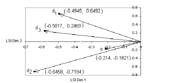
有了tf-idf值表示的文档向量，我们就可以训练一个LSI模型，和Latent Semantic Indexing (LSI) A Fast Track Tutorial中的例子相似，我们设置topic数为2：

>>> lsi = models.LsiModel(corpus_tfidf, id2word=dictionary, num_topics=2)
>>> lsi.print_topics(2)
2013-05-27 19:15:26,467 : INFO : topic #0(1.137): 0.438*”gold” + 0.438*”shipment” + 0.366*”truck” + 0.366*”arrived” + 0.345*”damaged” + 0.345*”fire” + 0.297*”silver” + 0.149*”delivery” + 0.000*”in” + 0.000*”a”
2013-05-27 19:15:26,468 : INFO : topic #1(1.000): 0.728*”silver” + 0.364*”delivery” + -0.364*”fire” + -0.364*”damaged” + 0.134*”truck” + 0.134*”arrived” + -0.134*”shipment” + -0.134*”gold” + -0.000*”a” + -0.000*”in”

lsi的物理意义不太好解释，不过最核心的意义是将训练文档向量组成的矩阵SVD分解，并做了一个秩为2的近似SVD分解，可以参考那篇英文tutorail。有了这个lsi模型，我们就可以将文档映射到一个二维的topic空间中：

>>> corpus_lsi = lsi[corpus_tfidf]
>>> for doc in corpus_lsi:
… print doc
…
[(0, 0.67211468809878649), (1, -0.54880682119355917)]
[(0, 0.44124825208697727), (1, 0.83594920480339041)]
[(0, 0.80401378963792647)]

可以看出，文档1，3和topic1更相关，文档2和topic2更相关；

我们也可以顺手跑一个LDA模型：

>>> lda = models.LdaModel(copurs_tfidf, id2word=dictionary, num_topics=2)
>>> lda.print_topics(2)
2013-05-27 19:44:40,026 : INFO : topic #0: 0.119*silver + 0.107*shipment + 0.104*truck + 0.103*gold + 0.102*fire + 0.101*arrived + 0.097*damaged + 0.085*delivery + 0.061*of + 0.061*in
2013-05-27 19:44:40,026 : INFO : topic #1: 0.110*gold + 0.109*silver + 0.105*shipment + 0.105*damaged + 0.101*arrived + 0.101*fire + 0.098*truck + 0.090*delivery + 0.061*of + 0.061*in

lda模型中的每个主题单词都有概率意义，其加和为1，值越大权重越大，物理意义比较明确，不过反过来再看这三篇文档训练的2个主题的LDA模型太平均了，没有说服力。

好了，我们回到LSI模型，有了LSI模型，我们如何来计算文档直接的相思度，或者换个角度，给定一个查询Query，如何找到最相关的文档？当然首先是建索引了：

>>> index = similarities.MatrixSimilarity(lsi[corpus])
2013-05-27 19:50:30,282 : INFO : scanning corpus to determine the number of features
2013-05-27 19:50:30,282 : INFO : creating matrix for 3 documents and 2 features

还是以这篇英文tutorial中的查询Query为例：gold silver truck。首先将其向量化：

>>> query = “gold silver truck”
>>> query_bow = dictionary.doc2bow(query.lower().split())
>>> print query_bow
[(3, 1), (9, 1), (10, 1)]

再用之前训练好的LSI模型将其映射到二维的topic空间：

>>> query_lsi = lsi[query_bow]
>>> print query_lsi
[(0, 1.1012835748628467), (1, 0.72812283398049593)]

最后就是计算其和index中doc的余弦相似度了：

>>> sims = index[query_lsi]
>>> print list(enumerate(sims))
[(0, 0.40757114), (1, 0.93163693), (2, 0.83416492)]

当然，我们也可以按相似度进行排序：

>>> sort_sims = sorted(enumerate(sims), key=lambda item: -item[1])
>>> print sort_sims
[(1, 0.93163693), (2, 0.83416492), (0, 0.40757114)]

可以看出，这个查询的结果是doc2 > doc3 > doc1，和fast tutorial是一致的，虽然数值上有一些差别：

好了，这个例子就到此为止，下一节我们将主要说明如何基于gensim计算课程图谱上课程之间的主题相似度，同时考虑一些改进方法，包括借助英文的自然语言处理工具包NLTK以及用更大的维基百科的语料来看看效果。

三、课程图谱相关实验

1、数据准备
为了方便大家一起来做验证，这里准备了一份Coursera的课程数据，可以在这里下载：coursera_corpus，（百度网盘链接: http://t.cn/RhjgPkv，密码: oppc）总共379个课程，每行包括3部分内容：课程名\t课程简介\t课程详情, 已经清除了其中的html tag, 下面所示的例子仅仅是其中的课程名：

Writing II: Rhetorical Composing
Genetics and Society: A Course for Educators
General Game Playing
Genes and the Human Condition (From Behavior to Biotechnology)
A Brief History of Humankind
New Models of Business in Society
Analyse Numérique pour Ingénieurs
Evolution: A Course for Educators
Coding the Matrix: Linear Algebra through Computer Science Applications
The Dynamic Earth: A Course for Educators
…

好了，首先让我们打开Python, 加载这份数据：

>>> courses = [line.strip() for line in file(‘coursera_corpus’)]
>>> courses_name = [course.split(‘\t’)[0] for course in courses]
>>> print courses_name[0:10]
[‘Writing II: Rhetorical Composing’, ‘Genetics and Society: A Course for Educators’, ‘General Game Playing’, ‘Genes and the Human Condition (From Behavior to Biotechnology)’, ‘A Brief History of Humankind’, ‘New Models of Business in Society’, ‘Analyse Num\xc3\xa9rique pour Ing\xc3\xa9nieurs’, ‘Evolution: A Course for Educators’, ‘Coding the Matrix: Linear Algebra through Computer Science Applications’, ‘The Dynamic Earth: A Course for Educators’]

2、引入NLTK
NTLK是著名的Python自然语言处理工具包，但是主要针对的是英文处理，不过课程图谱目前处理的课程数据主要是英文，因此也足够了。NLTK配套有文档，有语料库，有书籍，甚至国内有同学无私的翻译了这本书: 用Python进行自然语言处理，有时候不得不感慨：做英文自然语言处理的同学真幸福。

首先仍然是安装NLTK，在NLTK的主页详细介绍了如何在Mac, Linux和Windows下安装NLTK：http://nltk.org/install.html ，最主要的还是要先装好依赖NumPy和PyYAML，其他没什么问题。安装NLTK完毕，可以import nltk测试一下，如果没有问题，还有一件非常重要的工作要做，下载NLTK官方提供的相关语料：

>>> import nltk
>>> nltk.download()

这个时候会弹出一个图形界面，会显示两份数据供你下载，分别是all-corpora和book，最好都选定下载了，这个过程需要一段时间，语料下载完毕后，NLTK在你的电脑上才真正达到可用的状态，可以测试一下布朗语料库：

>>> from nltk.corpus import brown
>>> brown.readme()
‘BROWN CORPUS\n\nA Standard Corpus of Present-Day Edited American\nEnglish, for use with Digital Computers.\n\nby W. N. Francis and H. Kucera (1964)\nDepartment of Linguistics, Brown University\nProvidence, Rhode Island, USA\n\nRevised 1971, Revised and Amplified 1979\n\nhttp://www.hit.uib.no/icame/brown/bcm.html\n\nDistributed with the permission of the copyright holder,\nredistribution permitted.\n’
>>> brown.words()[0:10]
[‘The’, ‘Fulton’, ‘County’, ‘Grand’, ‘Jury’, ‘said’, ‘Friday’, ‘an’, ‘investigation’, ‘of’]
>>> brown.tagged_words()[0:10]
[(‘The’, ‘AT’), (‘Fulton’, ‘NP-TL’), (‘County’, ‘NN-TL’), (‘Grand’, ‘JJ-TL’), (‘Jury’, ‘NN-TL’), (‘said’, ‘VBD’), (‘Friday’, ‘NR’), (‘an’, ‘AT’), (‘investigation’, ‘NN’), (‘of’, ‘IN’)]
>>> len(brown.words())
1161192

现在我们就来处理刚才的课程数据，如果按此前的方法仅仅对文档的单词小写化的话，我们将得到如下的结果：

>>> texts_lower = [[word for word in document.lower().split()] for document in courses]
>>> print texts_lower[0]
[‘writing’, ‘ii:’, ‘rhetorical’, ‘composing’, ‘rhetorical’, ‘composing’, ‘engages’, ‘you’, ‘in’, ‘a’, ‘series’, ‘of’, ‘interactive’, ‘reading,’, ‘research,’, ‘and’, ‘composing’, ‘activities’, ‘along’, ‘with’, ‘assignments’, ‘designed’, ‘to’, ‘help’, ‘you’, ‘become’, ‘more’, ‘effective’, ‘consumers’, ‘and’, ‘producers’, ‘of’, ‘alphabetic,’, ‘visual’, ‘and’, ‘multimodal’, ‘texts.’, ‘join’, ‘us’, ‘to’, ‘become’, ‘more’, ‘effective’, ‘writers…’, ‘and’, ‘better’, ‘citizens.’, ‘rhetorical’, ‘composing’, ‘is’, ‘a’, ‘course’, ‘where’, ‘writers’, ‘exchange’, ‘words,’, ‘ideas,’, ‘talents,’, ‘and’, ‘support.’, ‘you’, ‘will’, ‘be’, ‘introduced’, ‘to’, ‘a’, …

注意其中很多标点符号和单词是没有分离的，所以我们引入nltk的word_tokenize函数，并处理相应的数据：

>>> from nltk.tokenize import word_tokenize
>>> texts_tokenized = [[word.lower() for word in word_tokenize(document.decode(‘utf-8′))] for document in courses]
>>> print texts_tokenized[0]
[‘writing’, ‘ii’, ‘:’, ‘rhetorical’, ‘composing’, ‘rhetorical’, ‘composing’, ‘engages’, ‘you’, ‘in’, ‘a’, ‘series’, ‘of’, ‘interactive’, ‘reading’, ‘,’, ‘research’, ‘,’, ‘and’, ‘composing’, ‘activities’, ‘along’, ‘with’, ‘assignments’, ‘designed’, ‘to’, ‘help’, ‘you’, ‘become’, ‘more’, ‘effective’, ‘consumers’, ‘and’, ‘producers’, ‘of’, ‘alphabetic’, ‘,’, ‘visual’, ‘and’, ‘multimodal’, ‘texts.’, ‘join’, ‘us’, ‘to’, ‘become’, ‘more’, ‘effective’, ‘writers’, ‘…’, ‘and’, ‘better’, ‘citizens.’, ‘rhetorical’, ‘composing’, ‘is’, ‘a’, ‘course’, ‘where’, ‘writers’, ‘exchange’, ‘words’, ‘,’, ‘ideas’, ‘,’, ‘talents’, ‘,’, ‘and’, ‘support.’, ‘you’, ‘will’, ‘be’, ‘introduced’, ‘to’, ‘a’, …

对课程的英文数据进行tokenize之后，我们需要去停用词，幸好NLTK提供了一份英文停用词数据：

>>> from nltk.corpus import stopwords
>>> english_stopwords = stopwords.words(‘english’)
>>> print english_stopwords
[‘i’, ‘me’, ‘my’, ‘myself’, ‘we’, ‘our’, ‘ours’, ‘ourselves’, ‘you’, ‘your’, ‘yours’, ‘yourself’, ‘yourselves’, ‘he’, ‘him’, ‘his’, ‘himself’, ‘she’, ‘her’, ‘hers’, ‘herself’, ‘it’, ‘its’, ‘itself’, ‘they’, ‘them’, ‘their’, ‘theirs’, ‘themselves’, ‘what’, ‘which’, ‘who’, ‘whom’, ‘this’, ‘that’, ‘these’, ‘those’, ‘am’, ‘is’, ‘are’, ‘was’, ‘were’, ‘be’, ‘been’, ‘being’, ‘have’, ‘has’, ‘had’, ‘having’, ‘do’, ‘does’, ‘did’, ‘doing’, ‘a’, ‘an’, ‘the’, ‘and’, ‘but’, ‘if’, ‘or’, ‘because’, ‘as’, ‘until’, ‘while’, ‘of’, ‘at’, ‘by’, ‘for’, ‘with’, ‘about’, ‘against’, ‘between’, ‘into’, ‘through’, ‘during’, ‘before’, ‘after’, ‘above’, ‘below’, ‘to’, ‘from’, ‘up’, ‘down’, ‘in’, ‘out’, ‘on’, ‘off’, ‘over’, ‘under’, ‘again’, ‘further’, ‘then’, ‘once’, ‘here’, ‘there’, ‘when’, ‘where’, ‘why’, ‘how’, ‘all’, ‘any’, ‘both’, ‘each’, ‘few’, ‘more’, ‘most’, ‘other’, ‘some’, ‘such’, ‘no’, ‘nor’, ‘not’, ‘only’, ‘own’, ‘same’, ‘so’, ‘than’, ‘too’, ‘very’, ‘s’, ‘t’, ‘can’, ‘will’, ‘just’, ‘don’, ‘should’, ‘now’]
>>> len(english_stopwords)
127

总计127个停用词，我们首先过滤课程语料中的停用词：
>>> texts_filtered_stopwords = [[word for word in document if not word in english_stopwords] for document in texts_tokenized]
>>> print texts_filtered_stopwords[0]
[‘writing’, ‘ii’, ‘:’, ‘rhetorical’, ‘composing’, ‘rhetorical’, ‘composing’, ‘engages’, ‘series’, ‘interactive’, ‘reading’, ‘,’, ‘research’, ‘,’, ‘composing’, ‘activities’, ‘along’, ‘assignments’, ‘designed’, ‘help’, ‘become’, ‘effective’, ‘consumers’, ‘producers’, ‘alphabetic’, ‘,’, ‘visual’, ‘multimodal’, ‘texts.’, ‘join’, ‘us’, ‘become’, ‘effective’, ‘writers’, ‘…’, ‘better’, ‘citizens.’, ‘rhetorical’, ‘composing’, ‘course’, ‘writers’, ‘exchange’, ‘words’, ‘,’, ‘ideas’, ‘,’, ‘talents’, ‘,’, ‘support.’, ‘introduced’, ‘variety’, ‘rhetorical’, ‘concepts\xe2\x80\x94that’, ‘,’, ‘ideas’, ‘techniques’, ‘inform’, ‘persuade’, ‘audiences\xe2\x80\x94that’, ‘help’, ‘become’, ‘effective’, ‘consumer’, ‘producer’, ‘written’, ‘,’, ‘visual’, ‘,’, ‘multimodal’, ‘texts.’, ‘class’, ‘includes’, ‘short’, ‘videos’, ‘,’, ‘demonstrations’, ‘,’, ‘activities.’, ‘envision’, ‘rhetorical’, ‘composing’, ‘learning’, ‘community’, ‘includes’, ‘enrolled’, ‘course’, ‘instructors.’, ‘bring’, ‘expertise’, ‘writing’, ‘,’, ‘rhetoric’, ‘course’, ‘design’, ‘,’, ‘designed’, ‘assignments’, ‘course’, ‘infrastructure’, ‘help’, ‘share’, ‘experiences’, ‘writers’, ‘,’, ‘students’, ‘,’, ‘professionals’, ‘us.’, ‘collaborations’, ‘facilitated’, ‘wex’, ‘,’, ‘writers’, ‘exchange’, ‘,’, ‘place’, ‘exchange’, ‘work’, ‘feedback’]

停用词被过滤了，不过发现标点符号还在，这个好办，我们首先定义一个标点符号list:
>>> english_punctuations = [‘,’, ‘.’, ‘:’, ‘;’, ‘?’, ‘(‘, ‘)’, ‘[‘, ‘]’, ‘&’, ‘!’, ‘*’, ‘@’, ‘#’, ‘$’, ‘%’]

然后过滤这些标点符号：
>>> texts_filtered = [[word for word in document if not word in english_punctuations] for document in texts_filtered_stopwords]
>>> print texts_filtered[0]
[‘writing’, ‘ii’, ‘rhetorical’, ‘composing’, ‘rhetorical’, ‘composing’, ‘engages’, ‘series’, ‘interactive’, ‘reading’, ‘research’, ‘composing’, ‘activities’, ‘along’, ‘assignments’, ‘designed’, ‘help’, ‘become’, ‘effective’, ‘consumers’, ‘producers’, ‘alphabetic’, ‘visual’, ‘multimodal’, ‘texts.’, ‘join’, ‘us’, ‘become’, ‘effective’, ‘writers’, ‘…’, ‘better’, ‘citizens.’, ‘rhetorical’, ‘composing’, ‘course’, ‘writers’, ‘exchange’, ‘words’, ‘ideas’, ‘talents’, ‘support.’, ‘introduced’, ‘variety’, ‘rhetorical’, ‘concepts\xe2\x80\x94that’, ‘ideas’, ‘techniques’, ‘inform’, ‘persuade’, ‘audiences\xe2\x80\x94that’, ‘help’, ‘become’, ‘effective’, ‘consumer’, ‘producer’, ‘written’, ‘visual’, ‘multimodal’, ‘texts.’, ‘class’, ‘includes’, ‘short’, ‘videos’, ‘demonstrations’, ‘activities.’, ‘envision’, ‘rhetorical’, ‘composing’, ‘learning’, ‘community’, ‘includes’, ‘enrolled’, ‘course’, ‘instructors.’, ‘bring’, ‘expertise’, ‘writing’, ‘rhetoric’, ‘course’, ‘design’, ‘designed’, ‘assignments’, ‘course’, ‘infrastructure’, ‘help’, ‘share’, ‘experiences’, ‘writers’, ‘students’, ‘professionals’, ‘us.’, ‘collaborations’, ‘facilitated’, ‘wex’, ‘writers’, ‘exchange’, ‘place’, ‘exchange’, ‘work’, ‘feedback’]

更进一步，我们对这些英文单词词干化（Stemming)，NLTK提供了好几个相关工具接口可供选择，具体参考这个页面: http://nltk.org/api/nltk.stem.html , 可选的工具包括Lancaster Stemmer, Porter Stemmer等知名的英文Stemmer。这里我们使用LancasterStemmer:

>>> from nltk.stem.lancaster import LancasterStemmer
>>> st = LancasterStemmer()
>>> st.stem(‘stemmed’)
‘stem’
>>> st.stem(‘stemming’)
‘stem’
>>> st.stem(‘stemmer’)
‘stem’
>>> st.stem(‘running’)
‘run’
>>> st.stem(‘maximum’)
‘maxim’
>>> st.stem(‘presumably’)
‘presum’

让我们调用这个接口来处理上面的课程数据:
>>> texts_stemmed = [[st.stem(word) for word in docment] for docment in texts_filtered]
>>> print texts_stemmed[0]
[‘writ’, ‘ii’, ‘rhet’, ‘compos’, ‘rhet’, ‘compos’, ‘eng’, ‘sery’, ‘interact’, ‘read’, ‘research’, ‘compos’, ‘act’, ‘along’, ‘assign’, ‘design’, ‘help’, ‘becom’, ‘effect’, ‘consum’, ‘produc’, ‘alphabet’, ‘vis’, ‘multimod’, ‘texts.’, ‘join’, ‘us’, ‘becom’, ‘effect’, ‘writ’, ‘…’, ‘bet’, ‘citizens.’, ‘rhet’, ‘compos’, ‘cours’, ‘writ’, ‘exchang’, ‘word’, ‘idea’, ‘tal’, ‘support.’, ‘introduc’, ‘vary’, ‘rhet’, ‘concepts\xe2\x80\x94that’, ‘idea’, ‘techn’, ‘inform’, ‘persuad’, ‘audiences\xe2\x80\x94that’, ‘help’, ‘becom’, ‘effect’, ‘consum’, ‘produc’, ‘writ’, ‘vis’, ‘multimod’, ‘texts.’, ‘class’, ‘includ’, ‘short’, ‘video’, ‘demonst’, ‘activities.’, ‘envid’, ‘rhet’, ‘compos’, ‘learn’, ‘commun’, ‘includ’, ‘enrol’, ‘cours’, ‘instructors.’, ‘bring’, ‘expert’, ‘writ’, ‘rhet’, ‘cours’, ‘design’, ‘design’, ‘assign’, ‘cours’, ‘infrastruct’, ‘help’, ‘shar’, ‘expery’, ‘writ’, ‘stud’, ‘profess’, ‘us.’, ‘collab’, ‘facilit’, ‘wex’, ‘writ’, ‘exchang’, ‘plac’, ‘exchang’, ‘work’, ‘feedback’]

在我们引入gensim之前，还有一件事要做，去掉在整个语料库中出现次数为1的低频词，测试了一下，不去掉的话对效果有些影响：

>>> all_stems = sum(texts_stemmed, [])
>>> stems_once = set(stem for stem in set(all_stems) if all_stems.count(stem) == 1)
>>> texts = [[stem for stem in text if stem not in stems_once] for text in texts_stemmed]

3、引入gensim
有了上述的预处理，我们就可以引入gensim，并快速的做课程相似度的实验了。以下会快速的过一遍流程，具体的可以参考上一节的详细描述。

>>> from gensim import corpora, models, similarities
>>> import logging
>>> logging.basicConfig(format=’%(asctime)s : %(levelname)s : %(message)s’, level=logging.INFO)

>>> dictionary = corpora.Dictionary(texts)
2013-06-07 21:37:07,120 : INFO : adding document #0 to Dictionary(0 unique tokens)
2013-06-07 21:37:07,263 : INFO : built Dictionary(3341 unique tokens) from 379 documents (total 46417 corpus positions)

>>> corpus = [dictionary.doc2bow(text) for text in texts]

>>> tfidf = models.TfidfModel(corpus)
2013-06-07 21:58:30,490 : INFO : collecting document frequencies
2013-06-07 21:58:30,490 : INFO : PROGRESS: processing document #0
2013-06-07 21:58:30,504 : INFO : calculating IDF weights for 379 documents and 3341 features (29166 matrix non-zeros)

>>> corpus_tfidf = tfidf[corpus]

这里我们拍脑门决定训练topic数量为10的LSI模型：
>>> lsi = models.LsiModel(corpus_tfidf, id2word=dictionary, num_topics=10)

>>> index = similarities.MatrixSimilarity(lsi[corpus])
2013-06-07 22:04:55,443 : INFO : scanning corpus to determine the number of features
2013-06-07 22:04:55,510 : INFO : creating matrix for 379 documents and 10 features

基于LSI模型的课程索引建立完毕，我们以Andrew Ng教授的机器学习公开课为例，这门课程在我们的coursera_corpus文件的第211行，也就是：

>>> print courses_name[210]
Machine Learning

现在我们就可以通过lsi模型将这门课程映射到10个topic主题模型空间上，然后和其他课程计算相似度：
>>> ml_course = texts[210]
>>> ml_bow = dicionary.doc2bow(ml_course)
>>> ml_lsi = lsi[ml_bow]
>>> print ml_lsi
[(0, 8.3270084238788673), (1, 0.91295652151975082), (2, -0.28296075112669405), (3, 0.0011599008827843801), (4, -4.1820134980024255), (5, -0.37889856481054851), (6, 2.0446999575052125), (7, 2.3297944485200031), (8, -0.32875594265388536), (9, -0.30389668455507612)]
>>> sims = index[ml_lsi]
>>> sort_sims = sorted(enumerate(sims), key=lambda item: -item[1])

取按相似度排序的前10门课程：
>>> print sort_sims[0:10]
[(210, 1.0), (174, 0.97812241), (238, 0.96428639), (203, 0.96283489), (63, 0.9605484), (189, 0.95390636), (141, 0.94975704), (184, 0.94269753), (111, 0.93654782), (236, 0.93601125)]

第一门课程是它自己:
>>> print courses_name[210]
Machine Learning

第二门课是Coursera上另一位大牛Pedro Domingos机器学习公开课
>>> print courses_name[174]
Machine Learning

第三门课是Coursera的另一位创始人，同样是大牛的Daphne Koller教授的概率图模型公开课：
>>> print courses_name[238]
Probabilistic Graphical Models

第四门课是另一位超级大牛Geoffrey Hinton的神经网络公开课，有同学评价是Deep Learning的必修课。
>>> print courses_name[203]
Neural Networks for Machine Learning

感觉效果还不错，如果觉得有趣的话，也可以动手试试。