


接着上一篇手势数据集制作完成后,我们就能够根据数据集,然后模型构建,训练,保存,Board可视化。
代码中写出了相应的注释:
# coding: utf-8
# 读取.tfrecords格式数据集,进行geture的cnn构建、训练、模型保存
import tensorflow as tf
# 此实验将训练集和测试集微同一个集合
train_whole_sample_size = 16989 # 训练集总量
test_whole_sample_size = 16989 # 测试集总量
gesture_class = 9 # 分类类别个数
train_batch_size = 1000 # 训练集每个批次的样本个数
test_batch_size = 2000 # 测试集每个批次的样本个数
image_size = 28 # 样本size :28*28
# 训练集.tfrecords 路径
train_path = "my_tfrecords/gesture_train.tfrecords"
# tensorboard的graph文件 保存路径
graph_path = "my_graph/my_gra"
# CNN模型文件 保存路径
cnn_model_save_path = "cnn_model/cnn_model.ckpt"
print("/****************************/")
print(" gesture cnn train ~~~")
# function: 解码 .tfrecords文件
def read_and_decode(filename):
filename_queue = tf.train.string_input_producer([filename])
reader = tf.TFRecordReader()
_, serialized_example = reader.read(filename_queue)
features = tf.parse_single_example(
serialized_example,
features={
'label': tf.FixedLenFeature([], tf.int64),
'img_raw': tf.FixedLenFeature([], tf.string),
}
)
img = tf.decode_raw(features['img_raw'], tf.uint8) # 原图数据二进制解码为 无符号8位整型
img = tf.reshape(img, [image_size, image_size, 1]) # reshape 到原图size:28*28
img = tf.cast(img, tf.float32) * (1. / 255.) - 0.5 # 数据归一化
label = tf.cast(features['label'], tf.int64) # 获取样本对应的标签
return img, label # 返回样本及对应的标签
print("step 1 ~~~")
# function:加载tfrecords文件并进行文件解析
# train batch 训练集
img_train, labels_train = read_and_decode(train_path)
# 定义模型训练时的数据批次
img_train_batch, labels_train_batch = tf.train.shuffle_batch([img_train, labels_train],
batch_size=train_batch_size,
capacity=train_whole_sample_size,
min_after_dequeue=6000,
num_threads=2 # 线程数
)
train_labes = tf.one_hot(labels_train_batch, gesture_class, 1, 0) # label转为 one_hot格式
# test batch 测试集
img_test, labels_test = read_and_decode(train_path)
img_test_batch, labels_test_batch = tf.train.shuffle_batch([img_test, labels_test],
batch_size=test_batch_size,
capacity=test_whole_sample_size,
min_after_dequeue=1000,
num_threads=2 # 线程数
)
test_labes = tf.one_hot(labels_test_batch, gesture_class, 1, 0) # label转为 one_hot格式
print("step 2 ~~~")
# function:
# 初始化权值
# shape : 4D
def weight_variable(shape, f_name):
initial = tf.truncated_normal(shape, mean=0, stddev=0.1) # 生成截断的正太分布
return tf.Variable(initial, name=f_name)
# 初始化偏置
def bias_variable(shape, f_name):
initial = tf.constant(0.1, shape=shape) # 生成截断的正太分布
return tf.Variable(initial, name=f_name)
# 卷积层
def Conv2d_Filter(x, W):
# x :input tensor of shape [batch, in_height,in_width,in_channels]
# W :fliter / kernel tensor of shape [filter_height , filter_width , in_channels ,out_channels]
# strides[0]=strides[3]=1 ,strides[1]代表x方向步长,strides[2]代表y方向步长
# padding : A 'string' from: "SAME", "VALID"
return tf.nn.conv2d(x, W, strides=[1, 1, 1, 1], padding="SAME")
# max-pooling 池化层
def max_pooling_2x2(x):
# ksize [1,x,y,1] , 窗口大小
# strides[0]=strides[3]=1 ,strides[1]代表x方向步长,strides[2]代表y方向步长
return tf.nn.max_pool(x, ksize=[1, 2, 2, 1], strides=[1, 2, 2, 1], padding="SAME")
print("step 3 ~~~")
# function : 构建CNN模型
# 定义placeholder
# x:训练样本
# y:训练样本标签
x = tf.placeholder(tf.float32, [None, image_size, image_size, 1], name="images") # 注意:x的shape
y = tf.placeholder(tf.float32, [None, gesture_class], name="labels")
# 卷积层 1
with tf.name_scope('Conv1'):
W_conv1 = weight_variable([5, 5, 1, 32], 'W_conv1') # 1通道输入32通道输出
b_conv1 = bias_variable([32], 'b_conv1') # 32个输出对应32个偏置
with tf.name_scope('h_conv1'):
# 把单通道输入x进行卷积操作,加上偏置值通过relu函数激活,获得32个feature map
h_conv1 = tf.nn.relu(Conv2d_Filter(x, W_conv1) + b_conv1)
# 池化层 1
with tf.name_scope('Pool1'):
h_pool1 = max_pooling_2x2(h_conv1) # 进行 max_pooling
# 卷积层 2
with tf.name_scope('Conv2'):
W_conv2 = weight_variable([5, 5, 32, 64], 'W_conv2') # 32个通道输入,64通道输出
b_conv2 = bias_variable([64], 'b_conv2') # 64个输出对应64个偏置
with tf.name_scope('h_conv2'): # 把h_pool1通过卷积操作,加上偏置值,应用于 relu函数激活
h_conv2 = tf.nn.relu(Conv2d_Filter(h_pool1, W_conv2) + b_conv2)
# 池化层 2
with tf.name_scope('Pool2'):
h_pool2 = max_pooling_2x2(h_conv2) # 进行 max_pooling
# 28*28图片单通道数据输入
# 第一次卷积后图片size:28*28,输出32个feature map
# 第一次池化后变为size:14*14,仍为 32个feature map
# 第二次卷积后仍为14*14,输出的64个 feature map
# 第二次池化后为7*7 仍为 64个 feature map
# 7*7*64
# 全连接层 1
with tf.name_scope('Fc1'):
# 初始化第一个全连接层权值
W_fc1 = weight_variable([7 * 7 * 64, 1024], 'W_fc1') # 因为输入为 64张 size: 7*7 feature map,定义全连接层有1024个神经元
b_fc1 = bias_variable([1024], 'b_fc1') # 1024个节点
# 池化层的输出扁平化,变为1维张量
with tf.name_scope('Pool2_flat'):
h_pool2_flat = tf.reshape(h_pool2, [-1, 7 * 7 * 64])
# 全连接层的输出
with tf.name_scope('h_fc1'):
h_fc1 = tf.nn.relu(tf.matmul(h_pool2_flat, W_fc1) + b_fc1)
# keep_prob 用来表示神经元输出的更新概率
keep_prob = tf.placeholder(tf.float32, name="my_keep_prob")
h_fc1_drop = tf.nn.dropout(h_fc1, keep_prob, name="my_h_fc1_drop")
# 全连接层 2
with tf.name_scope('Fc2'):
# 第二个全连接层
W_fc2 = weight_variable([1024, gesture_class], 'W_fc2')
b_fc2 = bias_variable([gesture_class], 'b_fc2')
with tf.name_scope('softmax'):
prediction = tf.nn.softmax(tf.matmul(h_fc1_drop, W_fc2) + b_fc2, name="my_prediction")
# 交叉熵代价函数
with tf.name_scope('Corss_Entropy'):
corss_entropy = tf.reduce_mean(tf.nn.softmax_cross_entropy_with_logits(labels=y, logits=prediction),
name="loss") # 交叉熵
tf.summary.scalar('corss_entropy', corss_entropy) # 添加标量corss_entropy统计结果
# 使用Adam优化器进行迭代
with tf.name_scope('Train_step'):
train_step = tf.train.AdamOptimizer(1e-4).minimize(corss_entropy, name="train_step")
# 统计真实分类 和 预测分类
correct_prediction = tf.equal(tf.arg_max(prediction, 1), tf.arg_max(y, 1))
# 求准确率
accuracy = tf.reduce_mean(tf.cast(correct_prediction, tf.float32))
tf.summary.scalar('accuracy', accuracy) # 添加标量accuracy统计结果
# 为了生成汇总信息,需要运行所有这些节点,为避免冗繁的工作,
# 可以使用 tf.summary.merge_all() 来将op合并为一个操作
merged = tf.merge_all_summaries()
print("step 4 ~~~")
# In[7]:
# function: 训练模型
print("cnn train start ~~~")
with tf.Session() as sess: # 开始一个会话
init = tf.initialize_all_variables()
sess.run(init) # 变量初始化
# FileWriter 的构造函数中包含了参数log_dir,申明的所有事件都会写到它所指的目录下
train_writer = tf.train.SummaryWriter(graph_path, sess.graph); # 记录tensorflow graph
coord = tf.train.Coordinator() # 协同启动的线程
threads = tf.train.start_queue_runners(coord=coord, sess=sess) # 启动线程运行队列
saver = tf.train.Saver() # 模型保存
max_acc = 0 # 最高测试准确率测试
for i in range(1001):
img_xs, label_xs = sess.run([img_train_batch, train_labes]) # 读取训练 batch
sess.run(train_step, feed_dict={x: img_xs, y: label_xs, keep_prob: 0.75})
# loss_data=
# print(i,")Loss:", sess.run(loss,feed_dict={x:img_xs, y:label_xs, keep_prob: 1.0}))#?如果不打印是否会优化掉
if (i % 10) == 0:
print("训练第", i, "次")
img_test_xs, label_test_xs = sess.run([img_test_batch, test_labes]) # 读取测试 batch
acc = sess.run(accuracy, feed_dict={x: img_test_xs, y: label_test_xs, keep_prob: 1.0})
print("Itsers = " + str(i) + " 准确率: " + str(acc))
################################################
summay = sess.run(merged, feed_dict={x: img_test_xs, y: label_test_xs, keep_prob: 1})
# 每一次迭代中通过 add_summary 将测试得到的数据写入定义的 FileWriter
train_writer.add_summary(summay, i)
################################################
if max_acc < acc: # 记录测试准确率最大时的模型
max_acc = acc
saver.save(sess, save_path=cnn_model_save_path)
if acc > 0.996: # 达到这个准确率跳出训练循环
break
train_writer.close()
coord.request_stop()
coord.join(threads)
sess.close()
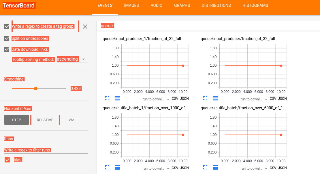
print("\n gesture cnn tfrecords 训练运行成功 ! ")代码中注释非常的清晰,在这里就不多叙了。其中,我们使用了TensorBoard进行显示一些graph和计算的图,
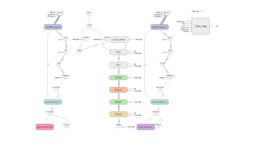
使用:tensorboard --logdir=file:///home/wuhao/PycharmProjects/tfrecord/my_graph/my_gra ,其中file为graph存放的位置,打开Board如下所示:
其中网络设计如下:


 5195
5195

 被折叠的 条评论
为什么被折叠?
被折叠的 条评论
为什么被折叠?
 到【灌水乐园】发言


