Coursera | Andrew Ng (01-week-2-2.10)— m 个样本的梯度下降

该系列仅在原课程基础上部分知识点添加个人学习笔记，或相关推导补充等。如有错误，还请批评指教。在学习了 Andrew Ng 课程的基础上，为了更方便的查阅复习，将其整理成文字。因本人一直在学习英语，所以该系列以英文为主，同时也建议读者以英文为主，中文辅助，以便后期进阶时，为学习相关领域的学术论文做铺垫。- ZJ

Coursera 课程 |deeplearning.ai |网易云课堂

---

转载请注明作者和出处：ZJ 微信公众号-「SelfImprovementLab」

知乎：https://zhuanlan.zhihu.com/c_147249273

CSDN：http://blog.csdn.net/JUNJUN_ZHAO/article/details/78922584

---

2.10 Gradient Descent on m examples

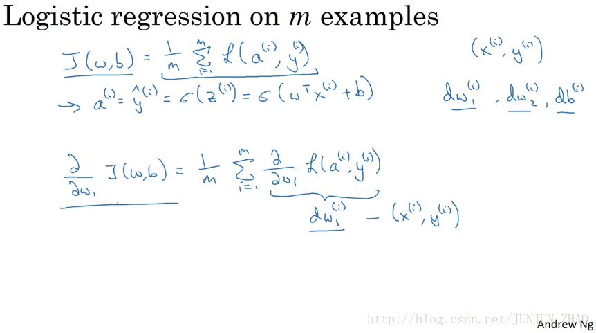
In the previous video you saw how to compute derivatives,and implement gradient descent with respect to just one training example for $logistic$ regression,now we want to do it for m training examples to get started,let’s remind ourselves that the definition of the cost function J cost function (w,b),which you care about is this average right,1 over m sum from i equals 1 through m,you know the loss when your algorithm output a^i on the example y well you know,a^i is the prediction on the I’ve trained example,which is $sigmoid$ of $z^i$,which is equal to $sigmoid$ of W transpose $x^i$plus b.

在之前的视频中你 已经看到如何计算导数和把梯度下降法应用到$logistic$回归的一个训练样本上 ，现在我们 想要把它应用在 m 个训练样本上，首先,时刻记住有关于，成本函数$J(w,b)$的定义，它是这样一个平均值，1/m 从 i=i 到 m 求和，这个损失函数 $L$ 当你的算法，在样本 (x,y) 输出了 $a^i$，你知道 $a^i$ 是训练样本的预测值，也就是$sigmoid(z^i)$，等于$sigmoid$作用于 $w$ 的转置 乘上$x^i$加上 $b$。

ok so what we show in the previous slide is for any single training example how to compute the derivatives,when you have just one training example,great so $dw_1$ $dw_2$ and $db$ with now the superscript i to denote the corresponding values you get,if you are doing what we did on the previous slide,but just using the one training example (x^i,y^i),excuse me I missing i there as well so,now you know the overall cost functions with the sum,was really the average of the 1 over m term of the individual losses,so it turns out that the derivative respect to say $w_1$ of the overall cost function is also going to be the average of derivatives,respect to $w_1$ of the individual loss terms.

我们在前面的幻灯中展示的是，对于任意单个训练样本如何计算导数，当你只有一个训练样本，$dw_1$ $dw_2$和$db$添上上标 i，表示相应的值，如果你做的是和上一张幻灯中演示的那种情况，但只使用了一个 训练样本$(x^i,y^i)$，抱歉 我这里少了个 i 现在你知道，全局成本函数 是一个求和，实际上是 1 到 m 项 损失函数和的平均，它表明 全局成本函数 对$w_1$的导数，也同样是各项损失函数，对$w_1$导数的平均。

but previously we have already shown how to compute this term,as say $(dw_1)^i$right which we you know on the previous slide,show how the computes on a single training example,so what you need to do is really compute these own derivatives,as we showed on the previous training example,and average them and this will give you the overall gradient,that you can use to implement straight into gradient decent,so I know there was a lot of details,but let’s take all of this up,and wrap this up into a concrete algorithms,and what you should implement together,just $logistic$ regression with gradient descent working.

但之前我们已经演示了如何计算这项，也就是我所写的即之前幻灯中演示的，如何对单个训练样本进行计算，所以你真正需要做的是计算这些导数，如我们在之前的训练样本上做的，并且求平均 这会得到全局梯度值，你能够把它直接应用到梯度下降算法中，所以 这里有很多细节，但让我们把这些，装进一个具体的算法，同时你需要一起应用的，就是$logistic$回归和和梯度下降法。

so just what you can do,let’s initialize J equals 0,um… $dw_1$ equals 0 $dw_2$ equals 0 $db$ equals 0,and what we’re going to do,is use a for loop over the training set, and compute the derivatives to respect each training example,and then add them up all right,so see as we do it for i equals 1 through m,so m is the number of training examples,we compute $z^i$ equals w transpose $x^i$plus b um…,the prediction $a^i$ is equal to $sigmoid$ of $z^i$,and then you know let’s let’s add up J,J plus equals $(y^i)log(a^i$) um…,plus 1 minus y I log 1 minus a^i,and then put a negative sign in front of the whole thing.

因此你能做的，让我们初始化$J=0$，$dw_1$等于 0 $dw_2$等于 0 $db$等于 0，并且我们将要做的是使用一个，for 循环遍历训练集 同时，计算相应的每个训练样本的导数，然后把它们加起来，好了 如我们所做的让 i 等于 1 到m，m 正好是训练样本个数，我们计算$z^i$等于 w 的转置乘上$x^i$加上b，$a^i$的预测值等于σ($z^i$)，然后你知道 让我们加上$J$，$J$加等于$(y^i)log(a^i)$，加上$(1-y^i)log(1-a^i)$，然后加上一个负号在整个公式的前面。

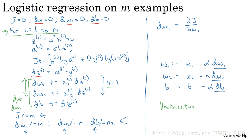
and then as we saw earlier we have $dz^i$,or it is equal to $a^i$ minus $y^i$ and $dw$,gets plus equals $(x_1)^i$ ，$dz^i$ $dw_2$ plus,equals $(x_2)^i$ $dz^i$ or and i’m doing this calculation,assuming that you have just the two features,so the n is equal to 2,otherwise you do this for $dw_1$ $dw_2$ $dw_3$ and so on,and $db$ plus equals $dz^i$,and I guess that’s the end of the for loop,and then finally having done this for all m training examples,you will still need to divide by m,because we’re computing averages,so $dw_1$ divide equals m $dw_2$ divide equals m,$db$ divide equals m in order to compute averages,and so with all of these calculations you’ve just computed,the derivative of the cost function J,with respect to each parameters $w_1$ $w_2$ and $b$.

我们之前见过 我们有$dz^i$，或者它等于$a^i$减去$y^i$ $dw$，加等于$(x_1)^i$乘上$dz^i$ $dw_2$加，等于$(x_2)^i$乘上$dz^i$ 或者我正在做这个计算，假设你只有两个特征，所以$n$等于 2，否则你做这个从$dw_1$ $dw_2$ $dw_3$ 一直下去，同时$db$加等于$dz^i$，我想 这是 for 循环的结束，最终对所有的 m 个训练样本都进行了这个计算，你还需要除以 m，因为我们计算平均值，因此$dw_1/=m$ $dw_2/=m$，$db/=m$ 可以计算平均值，随着所有这些计算 你已经计算了，损失函数J，对各个参数$w_1$ $w_2$和$b$的导数。

just come to details what we’re doing,we’re using $dw_1$ and $dw_2$ and $db$ to as accumulators right,so that after this computation you know,$dw_1$ is equal to the derivative of your overall cost function,with respect to $w_1$,and similarly for $dw_2$ and $db$ so notice that,$dw_1$ and $dw_2$ do not have a superscript i,because we’re using them in this code as accumulators,to sum over the entire training set whereas in contrast d$z^i$,here this was um… dz with respect to just one single training example,that is why that has a superscript i to refer to,the one training example i that’s computed on,and so having finished all these calculations,to implement one step of gradient descent you implement,$w_1$ gets updated as $w_1$ minus a learning rate times $dw_1$,$w_2$ gives updates as $w_2$ minus learning rate times $dw_2$,and b gets update as b minus learning rate times $db$,where $dw_1$ $dw_2$ and $db$ where you know as computed,and finally J here would also,be a correct value for your cost function.

回顾我们正在做的细节，我们使用$dw_1$ $dw_2$和$db$作为累加器，所以在这些计算之后，你知道$dw_1$等于你的全局成本函数，对$w_1$的导数，对$dw_2$和$db$也是一样 同时注意，$dw_1$和$dw_2$没有上标 i，因为我们在这代码中 把它们作为累加器，去求取整个训练集上的和 相反地 $dz^(i)$，这是对应于 单个训练样本的 $dz$，上标i指的是，对应第 i 个训练样本的计算，完成所有这些计算后，应用一步梯度下降，使得$w_1$获得更新 即$w_1$减去学习率乘上$dw_1$，$w_2$更新 即$w_2$减去 学习率乘上$dw_2$，同时更新 $b$ $b$ 减去学习率乘上$db$，这里$dw_1$ $dw_2$和$db$ 如你知道的被计算，最终这里的J也会，是你成本函数的正确值。

so everything on the slide implements,just one single step of gradient descent,and so you have to repeat everything on this slide multiple times,in order to take multiple steps of gradient descent,in case these details seem too complicated,again don’t worry too much about it,for now hopefully all this will be clearer,when you go and implement this in the programming assignment,but it turns out there are two weaknesses with the calculation,as with as with implements here,which is that to implement $logistic$ regression this way,you need to write two for loops the first for loop,is a small loop over the m training examples,and the second for loop is,a for loop over all the features over here,right so in this example we just had two features,so n is equal to 2 and n_x equals 2.

所以幻灯片上的所有东西，只应用了一次 梯度下降法，因此你需要 复以上内容很多次，以应用多次梯度下降，看起来这些细节 似乎很复杂，但目前不要担心太多，会清晰起来的，只要你在编程作业里 实现这些之后，但它表明计算中有两个缺点，当应用在这里的时候，就是说应用此方法到在$logistic$回归，你需要编写两个 for 循环 第一个 for 循环是，遍历 m 个训练样本的小循环，第二个 for 循环，是遍历所有特征的 for 循环，这个例子中 我们只有 2 个特征，所以 n 等于 2 $n_x$等于 2。

but if you have more features,you end up writing your $dw_1$ $dw_2$,and you have similar computations for $dw_3$,and so on down to $dw_n$,so seems like you need to,have a for loop over the features over all n features,when you’re implementing deep learning algorithms,you’ll find that having explicit for loops in your code,makes your algorithm run less efficiency,and so in the deep learning area,would move to a bigger and bigger data sets,and so being able to implement your algorithms,without using explicit for loops,is really important and will help you to scale to much bigger data sets,so it turns out that there are set of techniques called vectorization,techniques that allows you to get rid of these explicit for loops in your code.

但如果你有更多特征，你开始编写你的$dw_1$ $dw_2$，类似地计算$dw_3$，一直到$dw_n$，看来你需要一个 for 循环 遍历所有 n 个特征，当你应用深度学习算法，你会发现在代码中显式地使用for循环，会使算法很低效，同时在深度学习领域，会有越来越大的数据集，所以能够应用你的算法，完全不用显式 for 循环的话，会是重要的会帮助你，处理更大的数据集，有一门向量化技术，帮助你的代码 摆脱这些显式的for循环 。

I think in the pre deep learning era,that’s before the rise of deep learning,vectorization was a nice to have,you could sometimes do it to speed a vehicle,and sometimes not but in the deep learning era vectorization,that is getting rid of for loops like this,and like this has become really important,because we’re more and more training on very large datasets,and so you really need your code to be very efficient.

我想在深度学习时代的早期，也就是深度学习兴起之前，向量化是很棒的，有时候用来加速运算，但有时候也未必能够 但是在深度学习时代，用向量化来摆脱 for 循环，已经变得相当重要，因为我们越来越多地训练非常大的数据集，你的代码变需要得非常高效。

so in the next few videos we’ll talk aboutvectorization,and how to implement all this without using even a single for loop,so of this I hope you have a sense,of how to implement $logistic$ regression,or gradient descent for $logistic$ regression,um… things will be clearer when you implement the program exercise,but before actually doing the program exercise,let’s first talk about vectorization,so then you can implement this whole thing,implement a single iteration of gradient descent,without using any for loop

接下来的几个视频 我们会谈到向量化，以及如何应用这些 做到一个 for 循环都不需要使用，我希望你理解了，如何应用 $logistic$回归，对$logistic$回归应用梯度下降法，在你进行编程练习后应该会掌握得更清楚，但在做编程练习之前，让我们先谈谈“向量化”，然后你可以做到全部的这些，实现一个梯度下降法的迭代，而不需要 for 循环.。

---

重点总结：

m 个样本的梯度下降

对 m 个样本来说，其 Cost function 表达式如下：

$z^{(i)}= w^{T}x^{(i)}+b\\\hat y^{(i)}=a^{(i)}=\sigma(z^{(i)})\\J(w,b)=\dfrac{1}{m}\sum_{i=1}^{m}L(\hat y^{(i)}, y^{(i)})=-\dfrac{1}{m}\sum_{i=1}^{m}\left[y^{(i)}\log\hat y^{(i)}+(1-y^{(i)})\log(1-\hat y^{(i)})\right]$

Cost function 关于w和b的偏导数可以写成所有样本点偏导数和的平均形式：

$dw_{1} =\dfrac{1}{m}\sum_{i=1}^{m}x_{1}^{(i)}(a^{(i)}-y^{(i)})$

$db = \dfrac{1}{m}\sum_{i=1}^{m}(a^{(i)}-y^{(i)})$

参考文献：

[1]. 大树先生.吴恩达Coursera深度学习课程 DeepLearning.ai 提炼笔记（1-2）– 神经网络基础

---

PS: 欢迎扫码关注公众号：「SelfImprovementLab」！专注「深度学习」，「机器学习」，「人工智能」。以及 「早起」，「阅读」，「运动」，「英语 」「其他」不定期建群 打卡互助活动。