


最近在网易云课堂学习《深度学习》微专业,将课后的编程作业记录下来。
Logistic Regression with a Neural Network mindset
Welcome to your first (required) programming assignment! You will build a logistic regression classifier to recognize cats. This assignment will step you through how to do this with a Neural Network mindset, and so will also hone your intuitions about deep learning.
Instructions:
- Do not use loops (for/while) in your code, unless the instructions explicitly ask you to do so.
You will learn to:
- Build the general architecture of a learning algorithm, including:
- Initializing parameters
- Calculating the cost function and its gradient
- Using an optimization algorithm (gradient descent)
- Gather all three functions above into a main model function, in the right order.
程序
import numpy as np
import matplotlib.pyplot as plt
import h5py
import scipy
from PIL import Image
from scipy import ndimage
from lr_utils import load_dataset
## Loading the data (cat/non-cat)
train_set_x_orig, train_set_y, test_set_x_orig, test_set_y, classes = load_dataset()
## Data pre_processing
m_train = train_set_x_orig.shape[0]
m_test = test_set_x_orig.shape[0]
num_px = train_set_x_orig.shape[1]
train_set_x_flatten = train_set_x_orig.reshape(train_set_x_orig.shape[0],num_px*num_px*3).T
test_set_x_flatten = test_set_x_orig.reshape(test_set_x_orig.shape[0],num_px*num_px*3).T
train_set_x = train_set_x_flatten/255.
test_set_x = test_set_x_flatten/255.
## GRADED FUNCTION: sigmoid
def sigmoid(z):
"""
Compute the sigmoid of z
Arguments:
z -- A scalar or numpy array of any size.
Return:
s -- sigmoid(z)
"""
### START CODE HERE ### (≈ 1 line of code)
s = 1/(1+np.exp(-z))
### END CODE HERE ###
return s
## GRADED FUNCTION: initialize_with_zeros
def initialize_with_zeros(dim):
"""
This function creates a vector of zeros of shape (dim, 1) for w and initializes b to 0.
Argument:
dim -- size of the w vector we want (or number of parameters in this case)
Returns:
w -- initialized vector of shape (dim, 1)
b -- initialized scalar (corresponds to the bias)
"""
### START CODE HERE ### (≈ 1 line of code)
w = np.zeros(dim).reshape(dim,1)
# print("type of w:" + str(type(w)))
# print(w.shape)
b = 0
### END CODE HERE ###
assert(w.shape == (dim, 1))
assert(isinstance(b, float) or isinstance(b, int))
return w, b
## propagate FUNCTION: propagate to get the Y and cost
def propagate(w, b, X, Y):
"""
Implement the cost function and its gradient for the propagation explained above
Arguments:
w -- weights, a numpy array of size (num_px * num_px * 3, 1)
b -- bias, a scalar
X -- data of size (num_px * num_px * 3, number of examples)
Y -- true "label" vector (containing 0 if non-cat, 1 if cat) of size (1, number of examples)
Return:
cost -- negative log-likelihood cost for logistic regression
dw -- gradient of the loss with respect to w, thus same shape as w
db -- gradient of the loss with respect to b, thus same shape as b
Tips:
- Write your code step by step for the propagation. np.log(), np.dot()
"""
# print("w.shape="+str(w.shape))
# print("X.shape="+str(X.shape))
# print("Y.shape="+str(Y.shape))
m = X.shape[1]
# FORWARD PROPAGATION (FROM X TO COST)
### START CODE HERE ### (≈ 2 lines of code)
z = np.dot(w.T,X)+b
A = sigmoid(z) # compute activation
# print("z.shape="+str(z.shape))
# print("A.shape="+str(A.shape))
cost = -1/m * np.sum(np.dot(Y,np.log(A).T)+np.dot((1-Y),np.log(1-A).T)) # compute cost
### END CODE HERE ###
# BACKWARD PROPAGATION (TO FIND GRAD)
### START CODE HERE ### (≈ 2 lines of code)
dw = 1/m * (np.dot(X,(A-Y).T))
# print("dw.shape="+str(dw.shape))
db = 1/m * np.sum((A-Y),axis=1,keepdims=True)
### END CODE HERE ###
assert(dw.shape == w.shape)
assert(db.dtype == float)
cost = np.squeeze(cost)
assert(cost.shape == ())
grads = {"dw": dw,
"db": db}
return grads, cost
## GRADED FUNCTION: optimize
def optimize(w, b, X, Y, num_iterations, learning_rate, print_cost = False):
"""
This function optimizes w and b by running a gradient descent algorithm
Arguments:
w -- weights, a numpy array of size (num_px * num_px * 3, 1)
b -- bias, a scalar
X -- data of shape (num_px * num_px * 3, number of examples)
Y -- true "label" vector (containing 0 if non-cat, 1 if cat), of shape (1, number of examples)
num_iterations -- number of iterations of the optimization loop
learning_rate -- learning rate of the gradient descent update rule
print_cost -- True to print the loss every 100 steps
Returns:
params -- dictionary containing the weights w and bias b
grads -- dictionary containing the gradients of the weights and bias with respect to the cost function
costs -- list of all the costs computed during the optimization, this will be used to plot the learning curve.
Tips:
You basically need to write down two steps and iterate through them:
1) Calculate the cost and the gradient for the current parameters. Use propagate().
2) Update the parameters using gradient descent rule for w and b.
"""
costs = []
for i in range(num_iterations):
# Cost and gradient calculation (≈ 1-4 lines of code)
### START CODE HERE ###
grads, cost = propagate(w, b, X, Y)
### END CODE HERE ###
# Retrieve derivatives from grads
dw = grads["dw"]
db = grads["db"]
# update rule (≈ 2 lines of code)
### START CODE HERE ###
w = w - learning_rate * dw
b = b - learning_rate * b
### END CODE HERE ###
# Record the costs
if i % 100 == 0:
costs.append(cost)
# Print the cost every 100 training examples
if print_cost and i % 100 == 0:
print ("Cost after iteration %i: %f" %(i, cost))
params = {"w": w,
"b": b}
grads = {"dw": dw,
"db": db}
return params, grads, costs
## GRADED FUNCTION: predict
def predict(w, b, X):
'''
Predict whether the label is 0 or 1 using learned logistic regression parameters (w, b)
Arguments:
w -- weights, a numpy array of size (num_px * num_px * 3, 1)
b -- bias, a scalar
X -- data of size (num_px * num_px * 3, number of examples)
Returns:
Y_prediction -- a numpy array (vector) containing all predictions (0/1) for the examples in X
'''
m = X.shape[1]
Y_prediction = np.zeros((1,m))
w = w.reshape(X.shape[0], 1)
# Compute vector "A" predicting the probabilities of a cat being present in the picture
### START CODE HERE ### (≈ 1 line of code)
A = sigmoid(np.dot(w.T,X) + b)
# print(A)
### END CODE HERE ###
for i in range(A.shape[1]):
# Convert probabilities A[0,i] to actual predictions p[0,i]
### START CODE HERE ### (≈ 4 lines of code)
if A[0,i] > 0.5:
Y_prediction[0, i] = 1
else:
Y_prediction[0, i] = 0
### END CODE HERE ###
assert(Y_prediction.shape == (1, m))
return Y_prediction
## GRADED FUNCTION: model
def model(X_train, Y_train, X_test, Y_test, num_iterations = 2000, learning_rate = 0.5, print_cost = False):
"""
Builds the logistic regression model by calling the function you've implemented previously
Arguments:
X_train -- training set represented by a numpy array of shape (num_px * num_px * 3, m_train)
Y_train -- training labels represented by a numpy array (vector) of shape (1, m_train)
X_test -- test set represented by a numpy array of shape (num_px * num_px * 3, m_test)
Y_test -- test labels represented by a numpy array (vector) of shape (1, m_test)
num_iterations -- hyperparameter representing the number of iterations to optimize the parameters
learning_rate -- hyperparameter representing the learning rate used in the update rule of optimize()
print_cost -- Set to true to print the cost every 100 iterations
Returns:
d -- dictionary containing information about the model.
"""
### START CODE HERE ###
# initialize parameters with zeros (≈ 1 line of code)
w, b = initialize_with_zeros(X_train.shape[0])
# Gradient descent (≈ 1 line of code)
parameters, grads, costs = optimize(w, b, X_train, Y_train, num_iterations, learning_rate, print_cost = True)
# Retrieve parameters w and b from dictionary "parameters"
w = parameters["w"]
b = parameters["b"]
# Predict test/train set examples (≈ 2 lines of code)
Y_prediction_test = predict(w, b, X_test)
Y_prediction_train = predict(w, b, X_train)
### END CODE HERE ###
# Print train/test Errors
print("train accuracy: {} %".format(100 - np.mean(np.abs(Y_prediction_train - Y_train)) * 100))
print("test accuracy: {} %".format(100 - np.mean(np.abs(Y_prediction_test - Y_test)) * 100))
d = {"costs": costs,
"Y_prediction_test": Y_prediction_test,
"Y_prediction_train" : Y_prediction_train,
"w" : w,
"b" : b,
"learning_rate" : learning_rate,
"num_iterations": num_iterations}
return d
## test
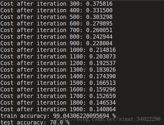
d = model(train_set_x, train_set_y, test_set_x, test_set_y, num_iterations = 2000, learning_rate = 0.005, print_cost = True)
# Plot learning curve (with costs)
costs = np.squeeze(d['costs'])
plt.plot(costs)
plt.ylabel('cost')
plt.xlabel('iterations (per hundreds)')
plt.title("Learning rate =" + str(d["learning_rate"]))
plt.show()
learning_rates = [0.01, 0.001, 0.0001]
models = {}
for i in learning_rates:
print ("learning rate is: " + str(i))
models[str(i)] = model(train_set_x, train_set_y, test_set_x, test_set_y, num_iterations = 1500, learning_rate = i, print_cost = False)
print ('\n' + "-------------------------------------------------------" + '\n')
for i in learning_rates:
plt.plot(np.squeeze(models[str(i)]["costs"]), label= str(models[str(i)]["learning_rate"]))
plt.ylabel('cost')
plt.xlabel('iterations')
legend = plt.legend(loc='upper center', shadow=True)
frame = legend.get_frame()
frame.set_facecolor('0.90')
plt.show()结果
测试集和训练集的预测结果
Comment: Training accuracy is close to 100%. This is a good sanity check: your model is working and has high enough capacity to fit the training data. Test error is 68%. It is actually not bad for this simple model, given the small dataset we used and that logistic regression is a linear classifier. But no worries, you’ll build an even better classifier next week!
Also, you see that the model is clearly overfitting the training data. Later in this specialization you will learn how to reduce overfitting, for example by using regularization. Using the code below (and changing the index variable) you can look at predictions on pictures of the test set.
梯度下降逐步优化损失函数
Interpretation:
You can see the cost decreasing. It shows that the parameters are being learned. However, you see that you could train the model even more on the training set. Try to increase the number of iterations in the cell above and rerun the cells. You might see that the training set accuracy goes up, but the test set accuracy goes down. This is called overfitting.
不同学习速率的结果对比
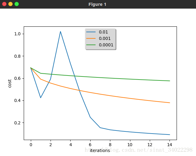
Interpretation:
- Different learning rates give different costs and thus different predictions results.
- If the learning rate is too large (0.01), the cost may oscillate up and down. It may even diverge (though in this example, using 0.01 still eventually ends up at a good value for the cost).
- A lower cost doesn’t mean a better model. You have to check if there is possibly overfitting. It happens when the training accuracy is a lot higher than the test accuracy.
- In deep learning, we usually recommend that you:
- Choose the learning rate that better minimizes the cost function.
- If your model overfits, use other techniques to reduce overfitting. (We’ll talk about this in later videos.)


 1218
1218


 被折叠的 条评论
为什么被折叠?
被折叠的 条评论
为什么被折叠?
 到【灌水乐园】发言


