机器学习算法与Python实践之（六）二分k均值聚类

zouxy09@qq.com

http://blog.csdn.net/zouxy09

 

       机器学习算法与python实践这个系列主要是参考《机器学习实战》这本书。因为自己想学习Python，然后也想对一些机器学习算法加深下了解，所以就想通过Python来实现几个比较常用的机器学习算法。恰好遇见这本同样定位的书籍，所以就参考这本书的过程来学习了。

       在上一个博文中，我们聊到了k-means算法。但k-means算法有个比较大的缺点就是对初始k个质心点的选取比较敏感。有人提出了一个二分k均值（bisecting k-means）算法，它的出现就是为了一定情况下解决这个问题的。也就是说它对初始的k个质心的选择不太敏感。那下面我们就来了解和实现下这个算法。

 

一、二分k均值（bisecting k-means）算法

       二分k均值（bisecting k-means）算法的主要思想是：首先将所有点作为一个簇，然后将该簇一分为二。之后选择能最大程度降低聚类代价函数（也就是误差平方和）的簇划分为两个簇。以此进行下去，直到簇的数目等于用户给定的数目k为止。

       以上隐含着一个原则是：因为聚类的误差平方和能够衡量聚类性能，该值越小表示数据点月接近于它们的质心，聚类效果就越好。所以我们就需要对误差平方和最大的簇进行再一次的划分，因为误差平方和越大，表示该簇聚类越不好，越有可能是多个簇被当成一个簇了，所以我们首先需要对这个簇进行划分。

       二分k均值算法的伪代码如下：

***************************************************************

将所有数据点看成一个簇

当簇数目小于k时

       对每一个簇

              计算总误差

              在给定的簇上面进行k-均值聚类（k=2）

              计算将该簇一分为二后的总误差

       选择使得误差最小的那个簇进行划分操作

***************************************************************

 

二、Python实现

       我使用的Python是2.7.5版本的。附加的库有Numpy和Matplotlib。具体的安装和配置见前面的博文。在代码中已经有了比较详细的注释了。不知道有没有错误的地方，如果有，还望大家指正（每次的运行结果都有可能不同）。里面我写了个可视化结果的函数，但只能在二维的数据上面使用。直接贴代码：

biKmeans.py

[python]  view plain  copy

1. #################################################  
2. # kmeans: k-means cluster  
3. # Author : zouxy  
4. # Date   : 2013-12-25  
5. # HomePage : http://blog.csdn.net/zouxy09  
6. # Email  : zouxy09@qq.com  
7. #################################################  
8.   
9. from numpy import *  
10. import time  
11. import matplotlib.pyplot as plt  
12.   
13.   
14. # calculate Euclidean distance  
15. def euclDistance(vector1, vector2):  
16.     return sqrt(sum(power(vector2 - vector1, 2)))  
17.   
18. # init centroids with random samples  
19. def initCentroids(dataSet, k):  
20.     numSamples, dim = dataSet.shape  
21.     centroids = zeros((k, dim))  
22.     for i in range(k):  
23.         index = int(random.uniform(0, numSamples))  
24.         centroids[i, :] = dataSet[index, :]  
25.     return centroids  
26.   
27. # k-means cluster  
28. def kmeans(dataSet, k):  
29.     numSamples = dataSet.shape[0]  
30.     # first column stores which cluster this sample belongs to,  
31.     # second column stores the error between this sample and its centroid  
32.     clusterAssment = mat(zeros((numSamples, 2)))  
33.     clusterChanged = True  
34.   
35.     ## step 1: init centroids  
36.     centroids = initCentroids(dataSet, k)  
37.   
38.     while clusterChanged:  
39.         clusterChanged = False  
40.         ## for each sample  
41.         for i in xrange(numSamples):  
42.             minDist  = 100000.0  
43.             minIndex = 0  
44.             ## for each centroid  
45.             ## step 2: find the centroid who is closest  
46.             for j in range(k):  
47.                 distance = euclDistance(centroids[j, :], dataSet[i, :])  
48.                 if distance < minDist:  
49.                     minDist  = distance  
50.                     minIndex = j  
51.               
52.             ## step 3: update its cluster  
53.             if clusterAssment[i, 0] != minIndex:  
54.                 clusterChanged = True  
55.                 clusterAssment[i, :] = minIndex, minDist**2  
56.   
57.         ## step 4: update centroids  
58.         for j in range(k):  
59.             pointsInCluster = dataSet[nonzero(clusterAssment[:, 0].A == j)[0]]  
60.             centroids[j, :] = mean(pointsInCluster, axis = 0)  
61.   
62.     print 'Congratulations, cluster using k-means complete!'  
63.     return centroids, clusterAssment  
64.   
65. # bisecting k-means cluster  
66. def biKmeans(dataSet, k):  
67.     numSamples = dataSet.shape[0]  
68.     # first column stores which cluster this sample belongs to,  
69.     # second column stores the error between this sample and its centroid  
70.     clusterAssment = mat(zeros((numSamples, 2)))  
71.   
72.     # step 1: the init cluster is the whole data set  
73.     centroid = mean(dataSet, axis = 0).tolist()[0]  
74.     centList = [centroid]  
75.     for i in xrange(numSamples):  
76.         clusterAssment[i, 1] = euclDistance(mat(centroid), dataSet[i, :])**2  
77.   
78.     while len(centList) < k:  
79.         # min sum of square error  
80.         minSSE = 100000.0  
81.         numCurrCluster = len(centList)  
82.         # for each cluster  
83.         for i in range(numCurrCluster):  
84.             # step 2: get samples in cluster i  
85.             pointsInCurrCluster = dataSet[nonzero(clusterAssment[:, 0].A == i)[0], :]  
86.   
87.             # step 3: cluster it to 2 sub-clusters using k-means  
88.             centroids, splitClusterAssment = kmeans(pointsInCurrCluster, 2)  
89.   
90.             # step 4: calculate the sum of square error after split this cluster  
91.             splitSSE = sum(splitClusterAssment[:, 1])  
92.             notSplitSSE = sum(clusterAssment[nonzero(clusterAssment[:, 0].A != i)[0], 1])  
93.             currSplitSSE = splitSSE + notSplitSSE  
94.   
95.             # step 5: find the best split cluster which has the min sum of square error  
96.             if currSplitSSE < minSSE:  
97.                 minSSE = currSplitSSE  
98.                 bestCentroidToSplit = i  
99.                 bestNewCentroids = centroids.copy()  
100.                 bestClusterAssment = splitClusterAssment.copy()  
101.   
102.         # step 6: modify the cluster index for adding new cluster  
103.         bestClusterAssment[nonzero(bestClusterAssment[:, 0].A == 1)[0], 0] = numCurrCluster  
104.         bestClusterAssment[nonzero(bestClusterAssment[:, 0].A == 0)[0], 0] = bestCentroidToSplit  
105.   
106.         # step 7: update and append the centroids of the new 2 sub-cluster  
107.         centList[bestCentroidToSplit] = bestNewCentroids[0, :]  
108.         centList.append(bestNewCentroids[1, :])  
109.   
110.         # step 8: update the index and error of the samples whose cluster have been changed  
111.         clusterAssment[nonzero(clusterAssment[:, 0].A == bestCentroidToSplit), :] = bestClusterAssment  
112.   
113.     print 'Congratulations, cluster using bi-kmeans complete!'  
114.     return mat(centList), clusterAssment  
115.   
116. # show your cluster only available with 2-D data  
117. def showCluster(dataSet, k, centroids, clusterAssment):  
118.     numSamples, dim = dataSet.shape  
119.     if dim != 2:  
120.         print "Sorry! I can not draw because the dimension of your data is not 2!"  
121.         return 1  
122.   
123.     mark = ['or', 'ob', 'og', 'ok', '^r', '+r', 'sr', 'dr', '<r', 'pr']  
124.     if k > len(mark):  
125.         print "Sorry! Your k is too large! please contact Zouxy"  
126.         return 1  
127.   
128.     # draw all samples  
129.     for i in xrange(numSamples):  
130.         markIndex = int(clusterAssment[i, 0])  
131.         plt.plot(dataSet[i, 0], dataSet[i, 1], mark[markIndex])  
132.   
133.     mark = ['Dr', 'Db', 'Dg', 'Dk', '^b', '+b', 'sb', 'db', '<b', 'pb']  
134.     # draw the centroids  
135.     for i in range(k):  
136.         plt.plot(centroids[i, 0], centroids[i, 1], mark[i], markersize = 12)  
137.           
138.     plt.show()  

三、测试结果

      测试数据是二维的，共80个样本。有4个类。具体见上一个博文。

测试代码：

test_biKmeans.py

[python]  view plain  copy

1. #################################################  
2. # kmeans: k-means cluster  
3. # Author : zouxy  
4. # Date   : 2013-12-25  
5. # HomePage : http://blog.csdn.net/zouxy09  
6. # Email  : zouxy09@qq.com  
7. #################################################  
8.   
9. from numpy import *  
10. import time  
11. import matplotlib.pyplot as plt  
12.   
13. ## step 1: load data  
14. print "step 1: load data..."  
15. dataSet = []  
16. fileIn = open('E:/Python/Machine Learning in Action/testSet.txt')  
17. for line in fileIn.readlines():  
18.     lineArr = line.strip().split('\t')  
19.     dataSet.append([float(lineArr[0]), float(lineArr[1])])  
20.   
21. ## step 2: clustering...  
22. print "step 2: clustering..."  
23. dataSet = mat(dataSet)  
24. k = 4  
25. centroids, clusterAssment = biKmeans(dataSet, k)  
26.   
27. ## step 3: show the result  
28. print "step 3: show the result..."  
29. showCluster(dataSet, k, centroids, clusterAssment)  

      这里贴出两次的运行结果：

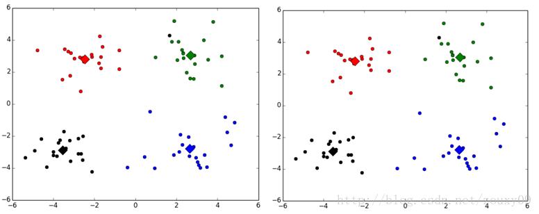
       不同的类用不同的颜色来表示，其中的大菱形是对应类的均值质心点。

       事实上，这个算法在初始质心选择不同时运行效果也会不同。我没有看初始的论文，不确定它究竟是不是一定会收敛到全局最小值。《机器学习实战》这本书说是可以的，但因为每次运行的结果不同，所以我有点怀疑，自己去找资料也没找到相关的说明。对这个算法有了解的还望您不吝指点下，谢谢。