


“CS 20SI: TensorFlow for Deep Learning Research”
Prepared by Chip Huyen
Reviewed by Danijar Hafner
Lecture note 4: How to structure your model in TensorFlow
个人翻译,部分内容较简略,建议参考原note阅读
本节课建立word2vec模型,不熟悉可以阅读CS224N的课件Mikolov的原始论文
Skip - gram模型 vs CBOW模型( Continuous Bag - of - Words):
算法上是相似的,不同的是CBOW根据上下文预测中心词,Skip-gram正好相反,统计上来讲,C通过把全部上下文当做一个观测值而使大量分布信息更为平滑,对于比较小的数据集这种方法很有用,S把(上下文-目标)对当做一个观测值,这使数据集更大的时候更有效
建立skip-gram模型,我们更关心隐藏层的权重,权重是我们所尝试学习的,也叫词向量矩阵
如何建造 tensorflow 模型
阶段1: 建造图:
- 定义输入输出的占位符
- 定义权重
- 定义模型inference
- 定义损失函数
- 定义optimizer
阶段2:执行计算:
- 给第一次执行初始变量
- feed训练数据,可能需要随机化数据样本
- 在训练数据下执行模型inference,计算当前输入和当前模型参数的输出
- 计算损失
- 通过最小/大化模型损失调整参数
让我们根据这些步骤穿件w2v,Skip-gram模型:
阶段1: 构造图:
- 定义输入输出的占位符
输入中心词,输出目标词,使用词列表索引代替one-hot向量,[batch_size]个标量输入和输出
center_words = tf.placeholder( tf.int32 , shape =[ BATCH_SIZE ]) target_words = tf.placeholder( tf.int32 , shape =[ BATCH_SIZE ])- 定义权重(词向量矩阵)
每行表示一个单词的词向量,每个词向量长度为EMBED_SIZE,那么词向量矩阵就是[VOCAB_SIZE,EMBED_SIZE],我们使用均匀分布初始化词向量矩阵
embed_matrix = tf.Variable(tf.random_uniform([ VOCAB_SIZE , EMBED_SIZE ], - 1.0 , 1.0 ))- inference(图前向传播通路)
tf.nn.embedding_lookup( params , ids , partition_strategy = 'mod' , name = None , validate_indices = True , max_norm = None)使用以上方法可以通过词向量矩阵转换单词索引为词向量
embed = tf.nn.embedding_lookup( embed_matrix , center_words)4 定义损失函数
NCE用py实现很复杂,tf自带的实现:
tf.nn.nce_loss( weights , biases , labels , inputs , num_sampled , num_classes , num_true = 1 , sampled_values = None , remove_accidental_hits = False , partition_strategy = 'mod' , name = 'nce_loss')我们需要隐藏层的权重和偏差去计算NCE损失
nce_weight = tf.Variable(tf.truncated_normal([VOCAB_SIZE, EMBED_SIZE],
                                                stddev=1.0 / (EMBED_SIZE ** 0.5)),
                                                name='nce_weight')
    nce_bias = tf.Variable(tf.zeros([VOCAB_SIZE]), name='nce_bias')
然后定义损失:
loss = tf.reduce_mean(tf.nn.nce_loss(weights=nce_weight,
                                        biases=nce_bias,
                                        labels=target_words,
                                        inputs=embed,
                                        num_sampled=NUM_SAMPLED,
num_classes=VOCAB_SIZE), name='loss')- 定义optimizer
optimizer = tf.train.GradientDescentOptimizer(LEARNING_RATE ).minimize(loss)阶段2:执行计算
建立session,给占位符feed输入和输出,运行优化器最小化loss,取回loss值
with tf.Session() as sess:
        sess.run(tf.global_variables_initializer())

        total_loss = 0.0 # we use this to calculate late average loss in the last SKIP_STEP steps
        writer = tf.summary.FileWriter('./my_graph/no_frills/', sess.graph)
        for index in xrange(NUM_TRAIN_STEPS):
            centers, targets = batch_gen.next()
            loss_batch, _ = sess.run([loss, optimizer],
                                    feed_dict={center_words: centers, target_words: targets})
            total_loss += loss_batch
            if (index + 1) % SKIP_STEP == 0:
                print('Average loss at step {}: {:5.1f}'.format(index, total_loss / SKIP_STEP))
                total_loss = 0.0
        writer.close()
nameScope
給张量命名并且在tensorboard中观察:
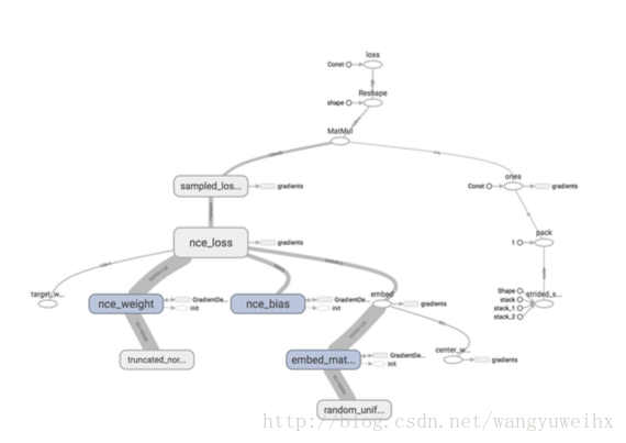
看起来乱七八糟的
使用tf.name_scope(name)将节点分类,节点会显示为一个scope,点击scope可以显示内部细节.你会发现tensorboard有节点两种线,一种是实线,另一种是虚线,实线代表数据流,虚线是节点所依赖的操作.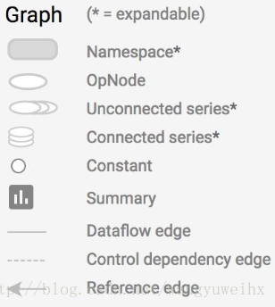
完整的节点图标
之前我们建立了一个简单的顺序模型,我们可以使用py的面向对象方法编写一个易于重用的模型,把Skip_gram建立为一个类:
class SkipGramModel:
    """ Build the graph for word2vec model """
    def __init__(self, vocab_size, embed_size, batch_size, num_sampled, learning_rate):
        self.vocab_size = vocab_size
        self.embed_size = embed_size
        self.batch_size = batch_size
        self.num_sampled = num_sampled
        self.lr = learning_rate
        self.global_step = tf.Variable(0, dtype=tf.int32, trainable=False, name='global_step')

    def _create_placeholders(self):
        """ Step 1: define the placeholders for input and output """
        with tf.name_scope("data"):
            self.center_words = tf.placeholder(tf.int32, shape=[self.batch_size], name='center_words')
            self.target_words = tf.placeholder(tf.int32, shape=[self.batch_size, 1], name='target_words')

    def _create_embedding(self):
        """ Step 2: define weights. In word2vec, it's actually the weights that we care about """
        # Assemble this part of the graph on the CPU. You can change it to GPU if you have GPU
        with tf.device('/cpu:0'):
            with tf.name_scope("embed"):
                self.embed_matrix = tf.Variable(tf.random_uniform([self.vocab_size,
                                                                    self.embed_size], -1.0, 1.0),
                                                                    name='embed_matrix')

    def _create_loss(self):
        """ Step 3 + 4: define the model + the loss function """
        with tf.device('/cpu:0'):
            with tf.name_scope("loss"):
                # Step 3: define the inference
                embed = tf.nn.embedding_lookup(self.embed_matrix, self.center_words, name='embed')

                # Step 4: define loss function
                # construct variables for NCE loss
                nce_weight = tf.Variable(tf.truncated_normal([self.vocab_size, self.embed_size],
                                                            stddev=1.0 / (self.embed_size ** 0.5)),
                                                            name='nce_weight')
                nce_bias = tf.Variable(tf.zeros([VOCAB_SIZE]), name='nce_bias')

                # define loss function to be NCE loss function
                self.loss = tf.reduce_mean(tf.nn.nce_loss(weights=nce_weight,
                                                    biases=nce_bias,
                                                    labels=self.target_words,
                                                    inputs=embed,
                                                    num_sampled=self.num_sampled,
                                                    num_classes=self.vocab_size), name='loss')
    def _create_optimizer(self):
        """ Step 5: define optimizer """
        with tf.device('/cpu:0'):
            self.optimizer = tf.train.GradientDescentOptimizer(self.lr).minimize(self.loss,
                                                              global_step=self.global_step)

    def _create_summaries(self):
        with tf.name_scope("summaries"):
            tf.summary.scalar("loss", self.loss)
            tf.summary.histogram("histogram loss", self.loss)
            # because you have several summaries, we should merge them all
            # into one op to make it easier to manage
            self.summary_op = tf.summary.merge_all()

    def build_graph(self):
        """ Build the graph for our model """
        self._create_placeholders()
        self._create_embedding()
        self._create_loss()
        self._create_optimizer()
        self._create_summaries()

def train_model(model, batch_gen, num_train_steps, weights_fld):
    saver = tf.train.Saver() # defaults to saving all variables - in this case embed_matrix, nce_weight, nce_bias

    initial_step = 0
    with tf.Session() as sess:
        sess.run(tf.global_variables_initializer())
        ckpt = tf.train.get_checkpoint_state(os.path.dirname('checkpoints/checkpoint'))
        # if that checkpoint exists, restore from checkpoint
        if ckpt and ckpt.model_checkpoint_path:
            saver.restore(sess, ckpt.model_checkpoint_path)

        total_loss = 0.0 # we use this to calculate late average loss in the last SKIP_STEP steps
        writer = tf.summary.FileWriter('improved_graph/lr' + str(LEARNING_RATE), sess.graph)
        initial_step = model.global_step.eval()
        for index in xrange(initial_step, initial_step + num_train_steps):
            centers, targets = batch_gen.next()
            feed_dict={model.center_words: centers, model.target_words: targets}
            loss_batch, _, summary = sess.run([model.loss, model.optimizer, model.summary_op],
                                              feed_dict=feed_dict)
            writer.add_summary(summary, global_step=index)
            total_loss += loss_batch
            if (index + 1) % SKIP_STEP == 0:
                print('Average loss at step {}: {:5.1f}'.format(index, total_loss / SKIP_STEP))
                total_loss = 0.0
                saver.save(sess, 'checkpoints/skip-gram', index)
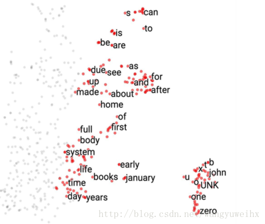
通过t-SNE我们可以把我们的词向量矩阵可视化,我们可以看到所有的数字被分类到右下角一行,挨着字母和名字,所有月份被分类到一组,所有”do,does,did”被分为一组等等.
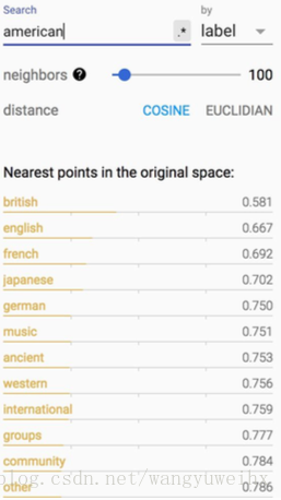
如果你打印’American’接近的词:
t - SNE(来自维基百科)
t - 分布随机相邻嵌入(t-SNE)是一种由Geoffrey Hinton和Laurens van der Maaten开发的机器学习降维算法。它是一种非线性降维技术,其特别适合将高维数据转换到二维或三维空间,然后以散点图可视化。具体来说,它通过一个二或三维空间来模拟每个高维对维点,使得类似对象由附近的点和不相似的对象的远近建模。t-SNE算法包括两个主要阶段。首先,t-SNE构建类似对象具有被选择的高概率,而不相似的点具有非常小被挑选的概率。第二,t-SNE定义了类似的概率分布低维地图中的点,并且在相对于地图中的点的位置的两个分布之间最小化Kullback-Leibler散度
我们也可以使用PCA使数据可视化
我们可以用不到十行的代码使数据可视化,tensorboard提供了很好的工具:
from tensorflow.contrib.tensorboard.plugins import projector
# obtain the embedding_matrix after you’ve trained it
final_embed_matrix = sess . run ( model . embed_matrix)
# create a variable to hold your embeddings. It has to be a variable. Constants
# don’t work. You also can’t just use the embed_matrix we defined earlier for our model. Why
# is that so? I don’t know. I get the 500 most popular words.
embedding_var = tf.Variable(final_embed_matrix[:500], name='embedding')
sess.run(embedding_var.initializer)
config = projector.ProjectorConfig()
summary_writer = tf.summary.FileWriter(LOGDIR)
# add embeddings to config
embedding = config.embeddings.add()
embedding.tensor_name = embedding_var.name
# link the embeddings to their metadata file. In this case, the file that contains
# the 500 most popular words in our vocabulary
embedding.metadata_path = LOGDIR + '/vocab_500.tsv'
# save a configuration file that TensorBoard will read during startup
projector.visualize_embeddings(summary_writer, config)
# save our embedding
saver_embed = tf.train.Saver([embedding_var])
saver_embed.save(sess, LOGDIR + '/skip-gram.ckpt', 1)
为什么我们依然要了解梯度
虽然目前为止我们建立的模型都没有获取单个节点的梯度,因为tf会自动考虑反向传播,但是我们依然要学会如何获取梯度,因为tf并不能分辨梯度消失或者梯度爆炸的情况,我们需要了解模型的梯度去获知模型是否正常工作


 2860
2860


 被折叠的 条评论
为什么被折叠?
被折叠的 条评论
为什么被折叠?
 到【灌水乐园】发言


