


 本文介绍了一个基于地理位置预测物种存在的模型。模型通过经纬度和时间输入,预测特定位置可能出现的物种,或为某一物种生成全球分布预测。支持两种运行模式:定位预测与地图预测。
目录
ReadMe
demo.py 是一个简单的demo,1)将位置作为输入,返回一个对所有分类是否会在该位置存在的预测,或2)为一个感兴趣的类别生成一个密集的预测。
geo_prior/ 地理先验,包括主要的训练和评估模型的代码gen_figs/ 生成图像,包括重新创建paper中的图像pre_process/ 预处理,包括训练图像分类器和保存特征/预测web_app/ 包括基于web的模型预测可视化的代码
demo.py
1)以一个位置作为输入,返回对每个类在这里存在的可能性的预测
或者2)以一个类别ID作为输入,为地球的每个位置生成一个预测
就是有两种方式,一种输入位置经纬度坐标,返回的是在这个位置,每个物种存在的概率,或者输入一个物种类别的ID,为地球上的每个经纬坐标生成该物种存在的预测。
import argparse
import numpy as np
import json
import matplotlib.pyplot as plt
import torch
import os
from six.moves import urllib

from geo_prior import models
from geo_prior import utils
from geo_prior import grid_predictor as grid
下载模型 download_model
def download_model(model_url, model_path):

    # Download pre-trained model if it is not currently available.
    if not os.path.isfile(model_path):
        try:
            print('Downloading model from: ' + model_url)
            urllib.request.urlretrieve(model_url, model_path)
        except:
            print('Failed to download model from: ' + model_url)
输入参数是model的url链接,和model的路径。这个函数用于模型目前不可用时,下载预训练的模型,如果该路径存在,则使用urllib.request.urlretrieve从传参的url链接下载模型。
主函数 main
def main(args):

    download_model(args.model_url, args.model_path)
    print('Loading model: ' + args.model_path)
    net_params = torch.load(args.model_path, map_location='cpu')
    params = net_params['params']
    model = models.FCNet(num_inputs=params['num_feats'], num_classes=params['num_classes'],
                         num_filts=params['num_filts'], num_users=params['num_users']).to(params['device'])
    model.load_state_dict(net_params['state_dict'])
    model.eval()
首先调用上面的download_model函数,接着从路径中加载下载的模型,调用models.FCNet。
# load class names
    with open(args.class_names_path) as da:
        class_data = json.load(da)
加载类名,这里有一个if-else分支,根据demo_type的不同,分为“location”和“map”。
如果是location:
- 通过调用utils中的encode_loc_time()函数,将经纬度坐标和时间整合到特征loc_time_feats。
- 打印“进行预测......”,调用model(loc_time_feats)进行预测。
- 这里设置num_categories=25,即显示Top 25个可能在该位置出现的物种。coords[0,0],coords[0,1]表示的是经纬度。对pred使用argsort()进行排序,并依次输出类id和类名。
if args.demo_type == 'location':
        # convert coords to torch  将坐标变换到torch
        coords = np.array([args.longitude, args.latitude])[np.newaxis, ...]
调用utils.py中的convert_loc_to_tensor,得到obs_coords:
obs_coords = utils.convert_loc_to_tensor(coords, params['device'])来看一下convert_loc_to_tensor()这个函数:它是将输入的经纬度进行规范化到[-1,1]的一个过程,再将规范化后的xt调用torch.from_numpy(),torch.from_numpy()方法把数组转换成张量,且二者共享内存,对张量进行修改比如重新赋值,那么原始数组也会相应发生改变。
def convert_loc_to_tensor(x, device=None):
    # intput is in lon {-180, 180}, lat {90, -90}
    xt = x.astype(np.float32)
    xt[:,0] /= 180.0
    xt[:,1] /= 90.0
    xt = torch.from_numpy(xt)
    if device is not None:
        xt = xt.to(device)
return xt 得到obs_time:调用torch.ones()(返回一个由标量值1填充的张量,其形状由变量参数size定义)
obs_time = torch.ones(coords.shape[0], device=params['device'])*args.time_of_year*2 - 1.0接下来将上面两步得到的obs_coords和obs_time作为输入,调用utils.py中的encode_loc_time()方法, 得到位置-时间特征loc_time_feats:
loc_time_feats = utils.encode_loc_time(obs_coords, obs_time, concat_dim=1, params=params)将得到的loc_time_feats输入模型中,得到预测,设置Top 25个类:
        print('Making prediction ...')
        with torch.no_grad():
            pred = model(loc_time_feats)[0, :]
        pred = pred.cpu().numpy()

        num_categories = 25
        print('\nTop {} likely categories for location {:.4f}, {:.4f}:'.format(num_categories, coords[0,0], coords[0,1]))
        most_likely = np.argsort(pred)[::-1]
        for ii, cls_id in enumerate(most_likely[:num_categories]):
            print('{}\t{}\t{:.3f}'.format(ii, cls_id, np.round(pred[cls_id], 3)) + \
'\t' + class_data[cls_id]['our_name'] + ' - ' + class_data[cls_id]['preferred_common_name'])如果demo_type是"map":为每个经纬度位置生成密集预测
- 如果没有指定感兴趣的类,就使用np.random.randint()随机选择一个
- 调用gp.dense_prediction()进行预测,传参包括模型,感兴趣的类,时间,结果保存在grid_pred。
- 调出该类的物种图片
- 调用plt.imsave()绘制热力图
    elif args.demo_type == 'map':
        # grid predictor - for making dense predictions for each lon/lat location
        gp = grid.GridPredictor(np.load('data/ocean_mask.npy'), params, mask_only_pred=True)
网格预测器,调用了grid_predictor.py中的GridPredictor()方法,GridPredictor(mask,paramsmask_only_pred=False),mask参数是载入了一个文件data/ocean_mask.npy隐藏了世界地图的海洋部分,mask_only_pred设置为True。
如果没有指定感兴趣的类,那么就随机指定一个。
        if args.class_of_interest == -1:
            args.class_of_interest = np.random.randint(len(class_data))
调用dense_prediction()方法进行预测
        print('Selected category: ' + class_data[args.class_of_interest]['our_name'] +\
            ' - ' + class_data[args.class_of_interest]['preferred_common_name'])

        print('Making prediction ...')
        grid_pred = gp.dense_prediction(model, args.class_of_interest, time_step=args.time_of_year)

        op_file_name = class_data[args.class_of_interest]['our_name'].lower().replace(' ', '_') + '.png'
        print('Saving prediction to: ' + op_file_name)
        plt.imsave(op_file_name, 1.0-grid_pred, cmap='afmhot', vmin=0, vmax=1
if __name__ == "__main__":
info_str = '\nPresence-Only Geographical Priors for Fine-Grained Image Classification.\n\n' + \
'This demo can be run in one of two ways:\n' + \
'1) Give a location and get a list of most likely classes there e.g\n' + \
' python demo.py location --longitude -118.1445155 --latitude 34.1477849 --time_of_year 0.5\n' + \
'Input coordinates should be in decimal degrees i.e. ' + \
'Longitude: [-180, 180], Latitude: [-90, 90], and Time of year [0, 1].\n\n' + \
'2) Give a category ID as input and get a prediction for each location on the globe for that category e.g.\n' + \
' python demo.py map --class_of_interest 3731\n' + \
'If class_of_interest is not specified a random one will be selected.\n\n'
model_path = 'models/model_inat_2018_full_final.pth.tar'
model_url = 'http://www.vision.caltech.edu/~macaodha/projects/geopriors/model_inat_2018_full_final.pth.tar'
class_names_path = 'web_app/data/categories2018_detailed.json'info_str:细粒度图像分类的仅存在地理先验。这个demo可以用以下两种方法的一种运行:
- 给定一个位置,得到一个最可能在这里存在的物种list。例如:
python demo.py location --longitude -118.1445155 --latitude 34.1477849 --time_of_year 0.5输入的坐标需要用数字表示经纬度,即Longitude:[-180,180],Ltitude:[-90,90],Time of year[0,1]
- 给定一个类别ID作为输入,得到全球每个位置上这个物种存在的预测。例如:
python demo.py map --class_of_interest 3731如果没有指定类别,就随机生成一个类ID。
运行结果
这是运行(1)中的示例指令的结果:生成了Top 25个在(-118.1445,34.1478)处可能存在的物种类别。

这是运行(2)示例指令的结果:
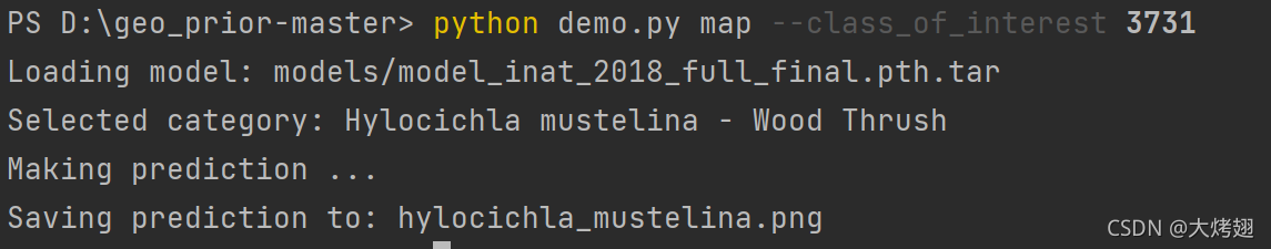
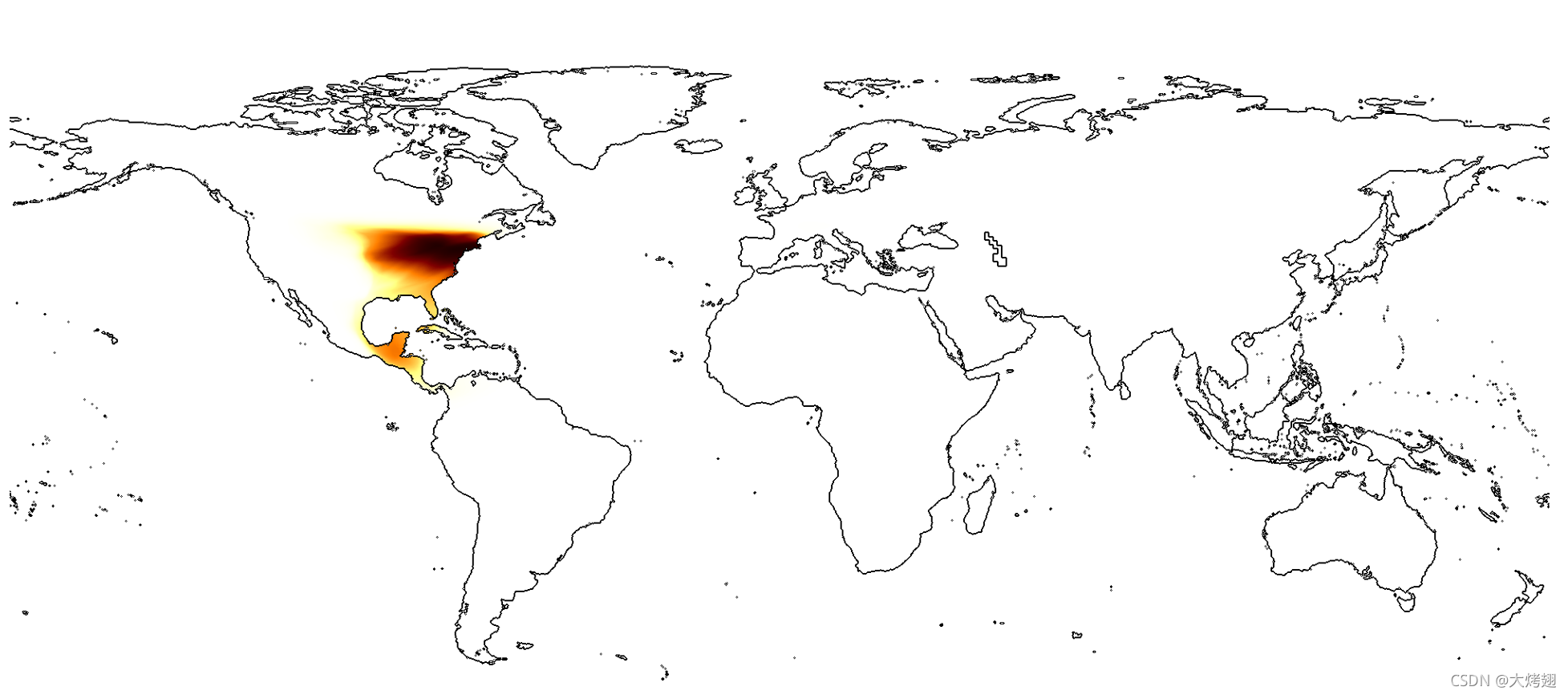
类别ID为3731的物种是Hylocichla mustelina - Wood Thrush,生成了一张图片hylocichla_mustelina.png,保存在项目根目录中,用来表示预测的分布,如下图。
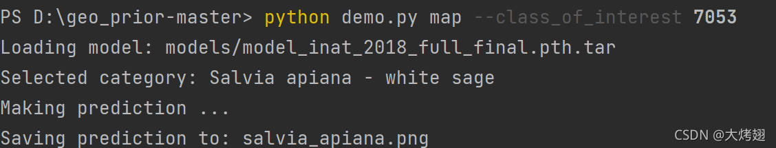
那么就想到将示例(1)的Top 1类别ID:7053 Salvia apiana - white sage作为输入,看看是什么结果:
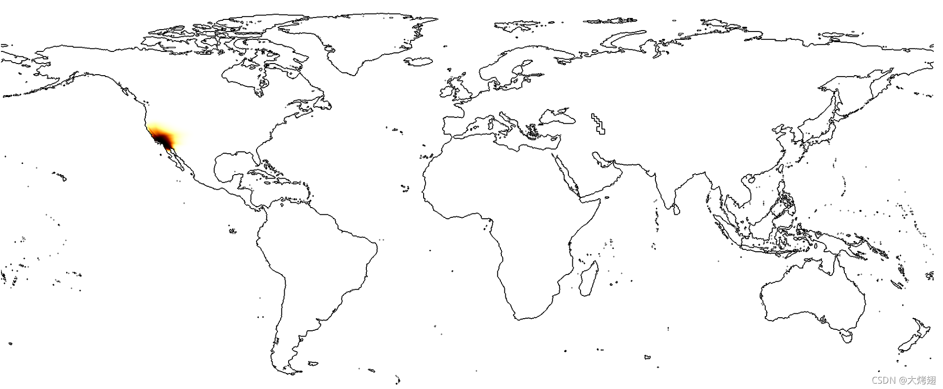 发现预测结果大概的位置正好与(1)中的输入差不多。
geo_prior/
Readme
train_geo_net.py 在不同数据集上训练我们的时空先验run_evaluation.py 为图像分类任务评估不同的先验
1.从我们的项目网页website中下载需要的数据集和元数据,将它们放在../data/目录下。这包括了特征和从训练的位置元数据图像分类器中提取的预测。你也需要为每iNat datasets数据集下载训练和验证文件。如果你想要评估现有的训练模型,确定你已经将它们放进了../models/
2.更新paths.py中的路径,让它们指向你的系统中正确的位置
3.确定你有requirements.txt中的包的版本。模型训练和评估在Python 3.7中展示。
Models.py
ResLayer类
class ResLayer(nn.Module):
    def __init__(self, linear_size):
        super(ResLayer, self).__init__()
        self.l_size = linear_size
        self.nonlin1 = nn.ReLU(inplace=True)
        self.nonlin2 = nn.ReLU(inplace=True)
        self.dropout1 = nn.Dropout()
        self.w1 = nn.Linear(self.l_size, self.l_size)
        self.w2 = nn.Linear(self.l_size, self.l_size)

    def forward(self, x):
        y = self.w1(x)
        y = self.nonlin1(y)
        y = self.dropout1(y)
        y = self.w2(y)
        y = self.nonlin2(y)
        out = x + y

        return out
FCNet类
class FCNet(nn.Module):
    def __init__(self, num_inputs, num_classes, num_filts, num_users=1):
        super(FCNet, self).__init__()
        self.inc_bias = False
        self.class_emb = nn.Linear(num_filts, num_classes, bias=self.inc_bias)
        self.user_emb = nn.Linear(num_filts, num_users, bias=self.inc_bias)

        self.feats = nn.Sequential(nn.Linear(num_inputs, num_filts),
                                    nn.ReLU(inplace=True),
                                    ResLayer(num_filts),
                                    ResLayer(num_filts),
                                    ResLayer(num_filts),
                                    ResLayer(num_filts))

    def forward(self, x, class_of_interest=None, return_feats=False):
        loc_emb = self.feats(x)
        if return_feats:
            return loc_emb
        if class_of_interest is None:
            class_pred = self.class_emb(loc_emb)
        else:
            class_pred = self.eval_single_class(loc_emb, class_of_interest)

        return torch.sigmoid(class_pred)

    def eval_single_class(self, x, class_of_interest):
        if self.inc_bias:
            return torch.matmul(x, self.class_emb.weight[class_of_interest, :]) + self.class_emb.bias[class_of_interest]
        else:
            return torch.matmul(x, self.class_emb.weight[class_of_interest, :])
Tang的方法
class TangNet(nn.Module):
    def __init__(self, ip_loc_dim, feats_dim, loc_dim, num_classes, use_loc):
        super(TangNet, self).__init__()
        self.use_loc  = use_loc
        self.fc_loc   = nn.Linear(ip_loc_dim, loc_dim)
        if self.use_loc:
            self.fc_class = nn.Linear(feats_dim+loc_dim, num_classes)
        else:
            self.fc_class = nn.Linear(feats_dim, num_classes)

    def forward(self, loc, net_feat):
        if self.use_loc:
            x = torch.sigmoid(self.fc_loc(loc))
            x = self.fc_class(torch.cat((x, net_feat), 1))
        else:
            x = self.fc_class(net_feat)
        return F.log_softmax(x, dim=1)


 901
901

 被折叠的 条评论
为什么被折叠?
被折叠的 条评论
为什么被折叠?
 到【灌水乐园】发言


