2.机器学习实战之K-近邻算法

最新推荐文章于 2024-05-20 10:26:35 发布

原创最新推荐文章于 2024-05-20 10:26:35 发布 · 1.3k 阅读

1 ·

CC 4.0 BY-SA版权

文章标签：

#K-近邻算法 #机器学习实战笔记

Machine Learning 专栏收录该内容

22 篇文章

订阅专栏

本文详细介绍了K-近邻算法的工作原理，包括欧氏距离的计算，以及算法的优缺点。通过伪代码展示了算法的执行过程，并提供了一个实际案例——用K-近邻算法改进约会网站的配对效果，包括数据预处理的文本转向量和归一化步骤，最后验证了算法的实施结果。

返回目录

1.简单理论介绍

1.1 k-近邻算法的工作原理

k-近邻算法（KNN）的工作原理是：我们有一个样本集，里面的每个数据都存在标签，即我们知道样本集中每一数据与所属分类的对应关系。输入没有标签的新数据后，依据数据的特征来计算新数据和样本集中数据的距离（这儿采用欧式距离），将计算后的距离按升序排序，选取距离最近的前k（一般小于20）个样本数据，将新数据的类别划分到这k个样本数据中所属类别最多的类。

1.2 欧氏距离

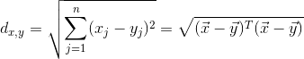
1.3 k-近邻算法优缺点

优点：精度高、对异常值不敏感、无数据输入假定

缺点：计算复杂度高、空间复杂度高、无法给出数据的基础结构信息

适用数据范围：数值型和标称型

2.伪代码

对未知类别属性的数据集中的每个点依次执行以下操作：

1)计算已知类别数据集中的点与当前点之间的距离；

2)按照距离递增次序排序；

3)选取与当前点距离最小的k个点；

4)确定前k个点所在类别的出现频率；

5)返回前k个点出现频率最高的类别作为当前点的预测分类。

3.算法实现

import numpy as np
import operator

# k-NearestNeighbor分类器
# inX：用于分类的输入向量(1xN)，dataSet：输入的训练样本(MxN)，labels：标签向量(1xM)，k：确定最后选择的最邻近邻居的数目。其中，M为样本数目，N为特征个数
def classify(inX,dataSet,labels,k):
    #计算欧式距离
    m = dataSet.shape[0]#得到输入训练样本的行数，即M
    diffMat = np.tile(inX,(m,1)) - dataSet#以inX为模板，复制M行，构成一个新的矩阵，然后减去训练样本矩阵
    sqDiffMat = diffMat**2
    sqDistances = sqDiffMat.sum(axis=1)# 1xM
    distances = sqDistances**0.5
    
    #选择距离最小的k个点
    sortedDistIndicies = distances.argsort()# 将距离进行排序，然后把排序后的距离原来位置的索引存入。
    classCount={}# dict
    for i in range(k):
        voteIlabel =labels[sortedDistIndicies[i]] # 得到所属标签
        classCount[voteIlabel] = classCount.get(voteIlabel,0) + 1# 将所属标签存入classCount字典中，以voteIlabel为健，以频数为值
    sortedClassCount = sorted(classCount.iteritems(),key=operator.itemgetter(1), reverse=True)# 将classCount转为iterable,指定以它的第二个域（即值）降序排序
    return sortedClassCount[0][0]

4. 测试算法

# 创建训练样本
def createDataSet():
    group = np.array([[1.0,1.1],[1.0,1.0],[0,0],[0,0.1]])
    labels = ['A','A','B','B']
    return group, labels

group,labels = createDataSet()
print 'group:',group
print 'labels:',labels

data = [0,0]# 新数据
data_label = classify(data,group,labels,3)
print 'data_label:',data_label

运行结果：

group: [[ 1.   1.1]
 [ 1.   1. ]
 [ 0.   0. ]
 [ 0.   0.1]]
labels: ['A', 'A', 'B', 'B']
data_label: B

5.示例：改进约会网站的配对效果

有1000行如下格式的数据：

40920	8.326976	0.953952	3
14488	7.153469	1.673904	2
26052	1.441871	0.805124	1
75136	13.147394	0.428964	1
38344	1.669788	0.134296	1
72993	10.141740	1.032955	1

前三列数据为特征，最后一列数据为类别。详细的来说，第一列数据表示每年获得的飞行常客里程数，第二列数据表示玩视频游戏所耗时间百分比，第三列数据表示每周消费的冰激凌公升数，现在要做的是根据这三个特征，来判断这个人所属类别。

5.1 将文本内容转为矩阵/向量

由于使用向量计算会提升速度，所以需要将文本内容转为向量格式。

代码实现：

#text-->matrix
#将文本转为特征矩阵和标签向量
#filename：数据文件路径
def file2matrix(filename):
    fr = open(filename)
    arrayOLines = fr.readlines()#一次读取所有内容，并按行将内容存入list
    numberOfLines = len(arrayOLines)#文件行数，这儿即训练样本个数M
    returnMat = np.zeros((numberOfLines,3))#创建一个M行，3列的矩阵
    classLabelVector = []
    index = 0
    for line in arrayOLines:
        line = line.strip()
        listFromLine = line.split('\t')
        returnMat[index,:] = listFromLine[0:3]# 将前3个元素存入到特征矩阵中
        classLabelVector.append(np.int(listFromLine[-1]))
        index += 1
    return returnMat,classLabelVector

path = r'D:\machine learning\machine learning in action\ch02\data\datingTestSet2.txt'
datingDataMat,datingLabels = file2matrix(path)

print 'data:',datingDataMat
print 'label:',datingLabels[:20]

运行结果：

data: [[  4.09200000e+04   8.32697600e+00   9.53952000e-01]
 [  1.44880000e+04   7.15346900e+00   1.67390400e+00]
 [  2.60520000e+04   1.44187100e+00   8.05124000e-01]
 ..., 
 [  2.65750000e+04   1.06501020e+01   8.66627000e-01]
 [  4.81110000e+04   9.13452800e+00   7.28045000e-01]
 [  4.37570000e+04   7.88260100e+00   1.33244600e+00]]
label: [3, 2, 1, 1, 1, 1, 3, 3, 1, 3, 1, 1, 2, 1, 1, 1, 1, 1, 2, 3]

5.2 归一化数据

由于第一个特征的的数值比第二个和第三个特征的数值大很多，为了避免这种情况对最后距离计算的影响，需要对数据进行归一化处理，即将所有数据归一化到0到1之间。归一化可以使用下面的公式：

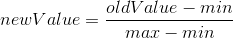
代码实现：

# normalization
# formula：newValue = (oldValue-min)/(max-min)
# dataSet:给定的数据集
def autoNorm(dataSet):
    minVals = dataSet.min(axis=0)#取得每个每一列的最小值，即每个特征中的最小值（1xN）
    maxVals = dataSet.max(axis=0)#取得每个每一列的最大值，即每个特征中的最大值（1xN）
    ranges = maxVals - minVals#得到每个特征的range（1xN）
    normDataSet = np.zeros(dataSet.shape)
    m = dataSet.shape[0]
    normDataSet = dataSet - np.tile(minVals,(m,1))# MxN
    normDataSet = normDataSet/np.tile(ranges,(m,1))# numpy“/”表示具体特征值相除
    return normDataSet,ranges,minVals

norMat,ranges,minVals = autoNorm(datingDataMat)
print 'norMat:',norMat
print 'ranges:',ranges
print 'minVals:',minVals

运行结果：

norMat: [[ 0.44832535  0.39805139  0.56233353]
 [ 0.15873259  0.34195467  0.98724416]
 [ 0.28542943  0.06892523  0.47449629]
 ..., 
 [ 0.29115949  0.50910294  0.51079493]
 [ 0.52711097  0.43665451  0.4290048 ]
 [ 0.47940793  0.3768091   0.78571804]]
ranges: [  9.12730000e+04   2.09193490e+01   1.69436100e+00]
minVals: [ 0.        0.        0.001156]

5.3 测试算法

def datingClassTest():
    hoRatio = 0.10    #使用90%的数据去训练，10%的数据去测试
    path = r'D:\machine learning\machine learning in action\ch02\data\datingTestSet2.txt'
    datingDataMat,datingLabels = file2matrix(path)       #load data setfrom file
    normMat, ranges, minVals = autoNorm(datingDataMat)
    m = normMat.shape[0]
    numTestVecs = int(m*hoRatio)
    errorCount = 0.0
    for i in range(numTestVecs):
        classifierResult = classify(normMat[i,:],normMat[numTestVecs:m,:],datingLabels[numTestVecs:m],3)
        print "the classifier came back with: %d, the real answer is: %d" % (classifierResult, datingLabels[i])
        if (classifierResult != datingLabels[i]): errorCount += 1.0
    print "the total error rate is: %f" % (errorCount/float(numTestVecs))
    print errorCount
    
datingClassTest()

运行结果：

the classifier came back with: 3, the real answer is: 3
the classifier came back with: 2, the real answer is: 3
the classifier came back with: 1, the real answer is: 1
the classifier came back with: 2, the real answer is: 2
the classifier came back with: 1, the real answer is: 1
the classifier came back with: 3, the real answer is: 3
the classifier came back with: 3, the real answer is: 3
...
the classifier came back with: 2, the real answer is: 2
the classifier came back with: 1, the real answer is: 1
the classifier came back with: 3, the real answer is: 1
the total error rate is: 0.050000
5.0

下一篇：决策树