representation learning 表示学习

representation learning

1. Review

2013年，Bengio等人发表了关于表示学习的综述[1]，摘要部分将无监督特征学习和深度学习的诸多进展纳入表示学习的范畴，做出三方面的尝试和贡献：第一，获取关于数据的表示需要考虑一些通用的先验；第二，为表示学习提供合适的目标函数；第三，厘清表示学习和其他机器学习任务的关系。原文如下：

The success of machine learning algorithms generally depends on data representation, and we hypothesize that this is because different representations can entangle and hide more or less the different explanatory factors of variation behind the data. Although specific domain knowledge can be used to help design representations, learning with generic priors can also be used, and the quest for AI is motivating the design of more powerful representation-learning algorithms implementing such priors. This paper reviews recent work in the area of unsupervised feature learning and deep learning, covering advances in probabilistic models, autoencoders, manifold learning, and deep networks. This motivates longer term unanswered questions about the appropriate objectives for learning good representations, for computing representations (i.e., inference), and the geometrical connections between representation learning, density estimation, and manifold learning.

2016年，Bengio和Goodfellow等人合著的《Deep Leanring》一书中，也为表示学习留了一章，内容不超出这篇综述。

1.1 WHAT

Bengio为表示学习下的定义是：

learning representations of the data that make it easier to extract useful information when building classifiers or other predictors

从这个定义可以看出，表示学习和后续的分类器（或者其他）是pipeline的过程，需要放在一起考虑，这一点对如何评价表示学习的性能也有决定性作用。

1.2 WHY

第一，从实践的角度来看，对于某些数据（尤其自然语言）来说，预处理和数据转换是必要的，传统的人工处理的方式费时费力。在包括语音信号处理、图像目标识别和自然语言处理等任务中，表示学习均取得了很多进展。

第二，在其他机器学习的问题应用中，表示学习也很重要。表示学习在迁移学习和领域自适应的任务中（注：迁移学习[transfer learning]侧重于不同任务间的转换，而领域自适应[domain adaption]侧重于输入具有不同的分布）取得的成功，证明了它能够真正学到数据背后的因素。

第三，文章把这个问题拔高到人工智能的终极目标的角度来看，认为要让AI彻底理解我们周围的世界，一个必要条件是它能从海量低层传感数据中发掘背后的解释性因子。

AI must fundamentally understand the world around us, and we argue that this can only be achieved if it can learn to identify and disentangle the underlying explanatory factors hidden in the observed milieu of low-level sensory data.

1.3 WHAT MAKES A REPRESENTATION GOOD?

为了获得一个好的表示，构建模型的时候需要正确反映一些对不同目标通用的先验知识。但是如何客观地评价一个表示的好坏是困难的，因为距离最终目标还隔着分类器等其他机器学习的任务，而且如何将这些先验形式化为一种评价准则仍然是一个开放的问题。

这些先验包括：

1. smoothness：记待估计的表示函数为$f$，$x≈y \rightarrow f(x)≈f(y)$；
   remark： 光滑性不足以解决维数灾难的问题，仅仅依靠对目标函数的光滑性假设做估计，就要求数据尽可能覆盖目标函数的空间。作为深度学习的三巨头之一，Bengio在本文又diss了一发核方法（kernel machine），因为核方法就建立在光滑性假设上，所以只能在简单的相似性度量适用的空间中使用。表示学习和核方法形成核学习，可以解决这个问题。
2. multiple explanatory factors：数据由不同的解释性因子决定，这些因子之间应该尽量解耦（disentangle）；
   remark： 分布式表示（distributed representation）。特征不变性和因子间解耦是有不同的：特征不变性砍掉了和任务无关的信息，但是很难预定义哪些特征和任务相关；因子间解耦则更加鲁棒，要求尽可能少地放弃信息。在不得不放弃一部分信息的时候，信息量最少的方向就被舍弃了（比如PCA就是这样的算法，各个维度之间相互正交，末尾的维度信息含量几乎可以忽略）。
3. hierarchical organization of explanatory factors：越抽象的概念在越高层
   remark： 深度表示。深度表示允许特征的复用，同时能够逐层抽象，又能够对输入的变化保持不变性（invariance）。特征的复用同时也是深度学习的核心优势，因为深层结构可以表示的函数族随着深度呈指数级上升，而相应增加的参数并不多。根据学习理论，小参数（尽管对比于传统方法，深度学习的参数量巨大，但是相比于能覆盖的函数族，参数量并不大）模型VC维小，所需要的样本量小（同样也是一种想蹲而言），计算效率和统计优势较大。
4. semi-supervised learning：现在有可以解释数据$X$分布的因子的子集，给定$X$的条件下，也需要能够解释目标$Y$。这就能够在无监督和有监督学习中起到共享统计优势的作用；
5. shared factors across tasks：解释性因子在其他任务中也有用；
6. manifolds：表示应该满足高维空间中的低维流形特点（简单来说，其含义就是虽然数据维数很高，但是聚集在维数远低于原空间的流形周围）；
   remark： 一些自动编码机算法（auto-encoder）
7. natural clustering：不同类的数据分布在分散的流形上，并且不同类数据的线性插值所处的区域密度低，也就是说$P(X|Y=i)$对不同的$i$良分离；
   remark： 流形相切算法（manifold tangent classifier）
8. temporal and spatial coherence：具有时空一致性的数据的类别概念相关，因此它们的表示相同或者仅仅在流形上有微小变化。可以对表示的该变量施加惩罚，从而获得平缓的变化；
9. sparsity：给定观测数据，其仅与一部分解释性因子相关，也即是说，在进行表示的时候，大部分特征都是0，或者在观测数据上的微小扰动对大部分特征是没有影响的。可以通过非线性操作（强制为0），惩罚梯度的Jacobian矩阵等方法实现；
   remark： 大部分特征为0的说法个人认为不太正确。考虑一个文本，用one-hot进行编码，其大部分的维度取值为0，但是改变其中一个单词（甚至是一个字母），就会造成编码较大的改变。
10. simplicity of factor dependencies：因子间的依赖关系简单。

2. word embedding

对于单词的表示方法而言，可以分成one-hot，continuous representation（比如Latent Semantic Analysis或者Latent Dirichlet Allocation）或者word-embedding。正如前文提到的，表示学习的一个难题在于缺乏完善的评价指标。评价词嵌入的效果有两类方法：

1. 提升现有系统性能，如将词向量用于文本分类、语义角色标注、词性标注等任务；
2. 语言学评价，类比方法详见2.2的结尾，可以类比的有语义关系、词法关系（例如单复数、比较级等）；

对于短语或者句子的表示，宏观来讲可以分成三种[4]：

1. Bag-of-Words（BoW）：广义上来讲，假设单词的表示和位置无关的都属于词袋模型。例如将单词的表示简单相加（或者取平均）；
2. Sequence：序列模型假设句子中的单词依赖于上下文；
3. Tree-structured：树结构模型将短语或者子分解为子短语或者子句的组合，这种组合具有固定的语法结构。

本节综述单词的表示方法，句子的表示方法留到下文。

2.1 Hinton 1986：Distributed representation

分布式表示的思想起源于Hinton 1986年的一个论文[3]，文章的后半部分全部是back-propagation的内容，几乎可以忽略；文章的前半部分举了不少实例来讨论如何用神经网络进行概念表示。

文章开门见山地指出在概念的表示有两个极端：一个是用单神经元表示每个概念，一个是用一组神经元去表示。二者是两种不同的语义理论的体现，结构主义者认为概念依赖于概念之间的相互关系得以定义，而不是依靠内在的本质，既然没有内在的本质，也就不需要用多个神经元进行表达；成分主义者认为概念由一组特征表达，所以在神经网络中，用神经元表达特征，概念是整个网络神经活动的稳定模式。当时沿着后者路线的研究工作存在的问题主要是：仅仅关心概念的相似性或者概念对的关联，没有概念如何扮演不同语法角色、如何进行因果推断给出明确的结构。

对此他讨论了两个方法：

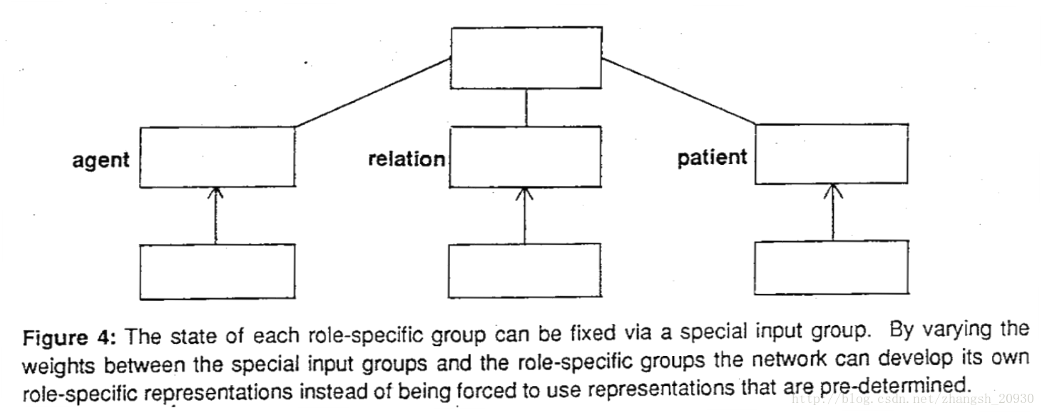
1. Role-specific units：对不同的概念，根据其不同的语法角色，给出不同的表示；缺点是参数太多，并且不能反映概念的关系。比如“John hit Mary”中John是主语（agent），“Mary divorced John”中John是宾语（patient），这种表示方法不能反映两个John之间的关系；
2. Conjunctive representation：首先考虑对概念使用相同的表示，再对语法角色进行表示，二者可以组合起来。比如前例中，（agent John）（relation hit）（patient Mary），这样的缺点是在做召回的时候，容易将（patient John）这样的命题召回，所以简单的组合也是有问题的。

既然全部给出不同的表示不行，简单组合也不行，那么就需要进行隐含特征的抽取，所以使用了神经网络如下。简单来说，文章的贡献在于通过线性映射（神经网络的主要操作）得到了隐含空间上的表达。

2.2 Bengio 2003：NNLM

词嵌入（word embedding）的经典之作是Bengio 2013年的论文[4]，其主要贡献在于开创了在训练语言模型的过程中“顺便”得到词向量的基本模型：neural network language model（NNLM）。

统计语言模型将单词出现的概率视为马尔可夫链，其每个单词的概率依赖于前面的所有单词：

$$\hat p(w^T_1)=\Pi_{t=1}^T \hat p(w_t|w_1^{t-1})$$

n-gram语法模型将依赖链缩减到前n-1个单词，即：

$$\hat p(w^{t-1}_1)=\hat p(w_t|w_{t-n+1}^{t-1})$$

论文提出了一个三层神经网络模型，对语言模型和词向量同时建模：

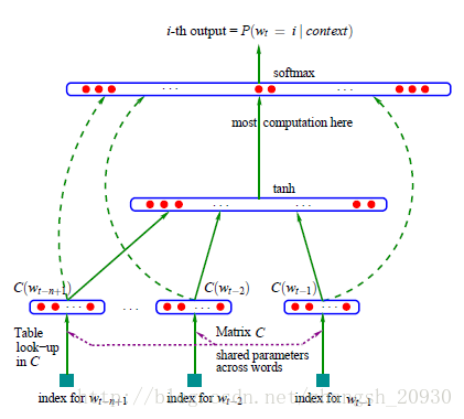
其中$C \in \mathcal{R}^{|V|*m}$存储了各个单词的词向量，$|V|$为字典大小，$m$为词向量的维度。输入是前n-1个词，输出是当前位置各个单词的概率。

网络将输入向量拼接，经过$\tanh(\cdot)$函数激活的神经网络；然后和跨层连接的输入向量相加，送入最后的softmax层：

$$y=softmax(b+W[C(w_{t-n+1}),...,C(w_{t-1})])+U\tanh(d+H[C(w_{t-n+1}),...,C(w_{t-1})])$$

训练的目标函数为负极大似然和正则项：

$$L=\frac{1}{T} \sum_t \log f(w_t, w_{t-1}, ..., w_{t-n+1}; \theta) + R(\theta)$$

评价指标为困惑度（perplexity），其基本思想是给测试集的句子赋予较高概率值的语言模型较好：

$$PP(W) = \left( \frac{1}{P \left( w_1,w_2,w_3,...,w_N \right)} \right)^{\frac{1}{N}}$$

在Brown语料库和Associated Press (AP) News语料库上效果远超传统n-gram模型。

NNLM的优点有：

1. 自带平滑特性（不需要传统n-gram语法模型对统计频率进行平滑的复杂技巧）；
2. 能够对字典外（out-of-vocabulary，oov）的单词进行建模并计算概率，即：

$$C(j)=\sum_i C(i) \hat p(i|w_{t-n+1}^{t-1})$$

文章的最后，Bengio充分发挥了挖坑的高超技巧，指出NNLM未来的几个方向，并且成功地“帮助”了若干学者毕业或者发出高质量文章，包括：

1. 可以用能量最小化，统一考虑输入向量和输出向量（[6,7]）；
2. 减少参数数量，例如采用循环神经网络（[8,9,10]）；
3. 网络分解、分层级等，加速网络训练（[7]）；
4. 词向量演示，揭示单词之间的关系，后来的工作一般都会证明符合这一点，例如：
   $$v(king)-v(queen)≈v(man)-v(woman)$$ 或者 $$@1[v(king)-v(man)+v(woman)] = v(queen)$$
   后者表示最近邻就是queen，比前者具有更强的语义。
5. 一词多义（[11]）

其影响力是当之无愧的。

2.3 Mnih & Hinton 2008 : Hierarchical Model

层次化softmax

2.4 Mikolov 2010-2011：RNNLM

2.5 Mikolov 2013：word2vec

注意到，原始NNLM其实可以拆分成两个步骤，第一步：用一个简单模型训练出连续的词向量；第二步，基于词向量的表达，训练一个连续的Ngram神经网络模型。原文如下：

…neural network language model can be successfully trained in two steps: first, continuous word vectors are learned using simple model, and then the N-gram NNLM is trained on top of these distributed representations of words.

而NNLM模型的计算瓶颈主要是在第二步，如果我们只是想得到word embeddings，应该对第二步进行简化。于是，Mikolov在文章[12]中提出两个模型：CBoW和Skip-gram model。二者的共同点在于对每个单词维护一个输入向量和一个输出向量（分别记为$V,U$）前者在给定上下文的情况下预测当前词，后者在给定当前词的情况下预测上下文。

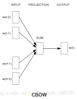
2.5.1 CBoW

Continuous Bag-of-Words Model（CBoW）相比于NNLM做出了一下三点改进：
1. 移除了非线性隐层；
2. 投影层对所有输入共享：在NNLM中，输入是拼接起来的，所以对不同单词而言，投影矩阵并不相同。为了实现共享，文章将输入直接求和。前文提到了，这种忽略了单词顺序的建模方法称为BoW，和传统BoW不同的是，这里的词向量是连续的，这就是模型明明为CBoW的原因；
3. 除了使用上文，文章也使用了下文，时间窗口是4。

优化log-linear分类器的输出概率（注：公式右端可以简化为线性项和log项相减，这也是log-linear得名的来源，为了保持可读性，这里保持分子分母的形式）：

$$\max \log p(w_t|w_{context}) = \log \frac{e^{U_t\cdot W\sum_{j\in context}V_j}}{\sum_k e^{U_k\cdot W\sum_{j\in context}V_j}}$$

可以看到，这事实上是在优化$w(t)$的输出向量和上下文的输入向量的投影之和的余弦相似度。

2.5.2 Skip-gram

Skip-gram model考虑当前单词对周围单词的预测，因为越远的单词相关性越弱，在采样的时候权重小，因此得名。

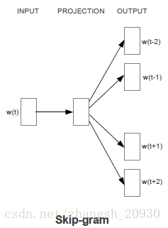
优化log-linear分类器的输出概率：

$$\max \log p(w_{context}|w_t) = \sum_{j \in context} \log \frac{e^{U_j V_t}}{\sum_k e^{U_k V_t}}=\sum_{j \in context}U_j V_t - \sum_{j\in context} \log \sum_k e^{U_k V_t}$$

上式的分母计算即使采用了Hierarchical softmax也极其费时，为此，Mikilov在[13]中提出若干优化技巧：

1. 对高频词下采样，加速效果在x2-x10之间，同时提高了低频词的准确性；
2. 负采样（Negative Sampling），提高高频词的准确性，同时加速训练，取得了比层次化softmax更快更好的效果；
3. 对固定搭配的短语看做一个单词，而非单词的组合，比如“Boston Probe”（一个报纸）的语义不能由“Boston”和“Probe”组合得到。

2.5.3 负采样

CBoW和Skip-gram的计算都很费时间，采用层次softmax可以加快训练，除此之外，Mikolov还提出了负采样的方法，取得了更快的速度和更好的性能。

负采样来源于Noise-Contrastive Estimation，原本是为了解决那些无法归一化的概率模型的参数预估问题。与改造模型输出概率的层次Softmax算法不同，NCE算法改造的是模型的似然函数：对于一组训练样本，上下文（或者当前词语）的出现，是来自于当前词语（或者上下文）的驱动，还是先验噪声的驱动？这个问题可以用一个Logistics回归来回答：

$$p(D=1|w_{context},w_t)=\frac{p(w_{context}|w_t)}{p(w_{context}|w_t)+k p_n(w_{context})}=\sigma \left( \log p(w_{context}|w_t) - \log k p_n(w_{context}) \right)$$

其中$k$是采样频率，$p_n(w_{context})$是噪声分布，简单地采用Logistics回归来代表上式的概率分布，可以得到：

$$\max \log p(w_{context}|w_t) = \sum_{j\in context}\log \sigma(U_j V_t) +\sum_{i=1}^k \mathbb{E}_{w_i \sim P_n(w)} \left[ \log \sigma(-U_{w_i} V_t) \right]$$

实际应用的过程中，对于小数据集 k <script type="math/tex" id="MathJax-Element-48">k</script>取5-20，对于大数据集取2-5足矣。

2.5.4 c代码解读

在读论文的过程中，对于具体怎么做分层softmax和负采样，还是有很多关于具体操作的困惑，源码google word2vec不是特别长，在这个博客中有一些解读。这里只列举最关键的部分。

    if (cbow)       //train the cbow architecture
    {  
      for (a = b; a < window * 2 + 1 - b; a++) if (a != window)//扫描目标单词的左右几个单词
      {
        c = sentence_position - window + a;
        if (c < 0) continue;
        if (c >= sentence_length) continue;
        last_word = sen[c];
        if (last_word == -1) continue;
        for (c = 0; c < layer1_size; c++)//layer1_size词向量的维度，默认值是100
            neu1[c] += syn0[c + last_word * layer1_size];//传说中的向量和？
      }
      if (hs) for (d = 0; d < vocab[word].codelen; d++)//开始遍历huffman树，每次一个节点
      {
        f = 0;
        l2 = vocab[word].point[d] * layer1_size;//point应该记录的是huffman的路径。找到当前节点，并算出偏移
        // Propagate hidden -> output
        for (c = 0; c < layer1_size; c++) f += neu1[c] * syn1[c + l2];//计算内积
        if (f <= -MAX_EXP) continue;//内积不在范围内直接丢弃
        else if (f >= MAX_EXP) continue;
        else f = expTable[(int)((f + MAX_EXP) * (EXP_TABLE_SIZE / MAX_EXP / 2))];//内积之后sigmoid函数
        // 'g' is the gradient multiplied by the learning rate
        g = (1 - vocab[word].code[d] - f) * alpha;//偏导数的一部分

        //layer1_size是向量的维度
        // Propagate errors output -> hidden 反向传播误差，从huffman树传到隐藏层。下面就是把当前内节点的误差传播给隐藏层，syn1[c + l2]是偏导数的一部分。
        for (c = 0; c < layer1_size; c++) neu1e[c] += g * syn1[c + l2];

        // Learn weights hidden -> output 更新当前内节点的向量，后面的neu1[c]其实是偏导数的一部分
        for (c = 0; c < layer1_size; c++) syn1[c + l2] += g * neu1[c];
      }
      // NEGATIVE SAMPLING
      if (negative > 0)
      for (d = 0; d < negative + 1; d++)
      {
        if (d == 0)
        {
          target = word;//目标单词
          label = 1;//正样本
        }
        else
        {
          next_random = next_random * (unsigned long long)25214903917 + 11;
          target = table[(next_random >> 16) % table_size];
          if (target == 0) target = next_random % (vocab_size - 1) + 1;
          if (target == word) continue;
          label = 0;//负样本
        }
        l2 = target * layer1_size;
        f = 0;
        for (c = 0; c < layer1_size; c++)
            f += neu1[c] * syn1neg[c + l2];//内积
        if (f > MAX_EXP)
            g = (label - 1) * alpha;
        else if (f < -MAX_EXP)
            g = (label - 0) * alpha;
        else g = (label - expTable[(int)((f + MAX_EXP) * (EXP_TABLE_SIZE / MAX_EXP / 2))]) * alpha;
        for (c = 0; c < layer1_size; c++)
            neu1e[c] += g * syn1neg[c + l2];//隐藏层的误差
        for (c = 0; c < layer1_size; c++)
            syn1neg[c + l2] += g * neu1[c];//更新负样本向量
      }
      // hidden -> in
      for (a = b; a < window * 2 + 1 - b; a++)
      if (a != window)//cbow模型 更新的不是中间词语的向量，而是周围几个词语的向量。
      {
        c = sentence_position - window + a;
        if (c < 0) continue;
        if (c >= sentence_length) continue;
        last_word = sen[c];
        if (last_word == -1) continue;
        for (c = 0; c < layer1_size; c++)
            syn0[c + last_word * layer1_size] += neu1e[c];//更新词向量
      }
    }
    else
    {  //train skip-gram
       for (a = b; a < window * 2 + 1 - b; a++)
       if (a != window)//扫描周围几个词语
       {
        c = sentence_position - window + a;
        if (c < 0) continue;
        if (c >= sentence_length) continue;
        last_word = sen[c];
        if (last_word == -1) continue;
        l1 = last_word * layer1_size;
        for (c = 0; c < layer1_size; c++)
            neu1e[c] = 0;
        // HIERARCHICAL SOFTMAX
        if (hs)
        for (d = 0; d < vocab[word].codelen; d++)//遍历叶子节点
        {
          f = 0;
          l2 = vocab[word].point[d] * layer1_size;//point记录的是huffman的路径
          // Propagate hidden -> output 感觉源代码这个英语注释有点误导人，这里的隐藏层就是输入层，就是词向量。
          for (c = 0; c < layer1_size; c++)
              f += syn0[c + l1] * syn1[c + l2];//计算两个词向量的内积
          if (f <= -MAX_EXP) continue;
          else if (f >= MAX_EXP) continue;
          else f = expTable[(int)((f + MAX_EXP) * (EXP_TABLE_SIZE / MAX_EXP / 2))];
          // 'g' is the gradient multiplied by the learning rate
          g = (1 - vocab[word].code[d] - f) * alpha;//偏导数的一部分
          // Propagate errors output -> hidden
          for (c = 0; c < layer1_size; c++)
              neu1e[c] += g * syn1[c + l2];//隐藏层的误差
          // Learn weights hidden -> output
          for (c = 0; c < layer1_size; c++)
              syn1[c + l2] += g * syn0[c + l1];//更新叶子节点向量
        }
        // NEGATIVE SAMPLING
        if (negative > 0)//这个同cobow差不多
        for (d = 0; d < negative + 1; d++)
        {
          if (d == 0)
          {
            target = word;
            label = 1;
          }
          else
          {
            next_random = next_random * (unsigned long long)25214903917 + 11;
            target = table[(next_random >> 16) % table_size];
            if (target == 0) target = next_random % (vocab_size - 1) + 1;
            if (target == word) continue;
            label = 0;
          }
          l2 = target * layer1_size;
          f = 0;
          for (c = 0; c < layer1_size; c++)
              f += syn0[c + l1] * syn1neg[c + l2];
          if (f > MAX_EXP) g = (label - 1) * alpha;
          else if (f < -MAX_EXP)
              g = (label - 0) * alpha;
          else g = (label - expTable[(int)((f + MAX_EXP) * (EXP_TABLE_SIZE / MAX_EXP / 2))]) * alpha;
          for (c = 0; c < layer1_size; c++)
              neu1e[c] += g * syn1neg[c + l2];
          for (c = 0; c < layer1_size; c++)
              syn1neg[c + l2] += g * syn0[c + l1];
        }

        // Learn weights input -> hidden
        for (c = 0; c < layer1_size; c++)
            syn0[c + l1] += neu1e[c];//更新周围几个词语的向量
      }
    }
    sentence_position++;
    if (sentence_position >= sentence_length)
    {
      sentence_length = 0;
      continue;
    }
  }

2.6 Kiros 2015： sent2vec

2.7 Jeffrey 2014：GloVe （and GloVe v.s. word2vec）

2.8 其他改进

3. language modelling and NLP tasks

Reference

1. [Bengio2013] Bengio Y, Courville A, Vincent P. Representation Learning: A Review and New Perspectives[J]. IEEE Transactions on Pattern Analysis & Machine Intelligence, 2013, 35(8):1798-1828.
2. [Goodfellow2016] Ian Goodfellow, Yoshua Bengio and Aaron Courville. Deep Learning, 2016, MIT Press. http://www.deeplearningbook.org/
3. [Hinton1986] Hinton G E. Learning distributed representations of concepts[C]//Proceedings of the eighth annual conference of the cognitive science society. 1986, 1: 12.
4. [Tai2015] Tai K S, Socher R, Manning C D. Improved Semantic Representations From Tree-Structured Long Short-Term Memory Networks[J]. Computer Science, 2015, 5(1): 36.
5. [Bengio2013] Yoshua Bengio, Rejean Ducharme, Pascal Vincent, and Christian Jauvin. A neural probabilistic language model. Journal of Machine Learning Research (JMLR), 3:1137–1155, 2003.
6. [Mnih2007] Andriy Mnih and Geoffrey Hinton. Three new graphical models for statistical language modelling. International Conference on Machine Learning (ICML). 2007.
7. [Mnih2008] Andriy Mnih & Geoffrey Hinton. A scalable hierarchical distributed language model. The Conference on Neural Information Processing Systems (NIPS) (pp. 1081–1088). 2008.
8. [Mikolov2010] Mikolov T, Karafiát M, Burget L, et al. Recurrent neural network based language model[C]//Interspeech. 2010, 2: 3.
9. [Mikolov2011] Mikolov T, Kombrink S, Burget L, et al. Extensions of recurrent neural network language model[C]//Acoustics, Speech and Signal Processing (ICASSP), 2011 IEEE International Conference on. IEEE, 2011: 5528-5531.
10. [Kombrink2011] Kombrink S, Mikolov T, Karafiát M, et al. Recurrent neural network based language modeling in meeting recognition[C]//Twelfth Annual Conference of the International Speech Communication Association. 2011.
11. [Huang2012] Eric Huang, Richard Socher, Christopher Manning and Andrew Ng. Improving word representations via global context and multiple word prototypes. Proceedings of the 50th Annual Meeting of the Association for Computational Linguistics: Long Papers-Volume 1. 2012.
12. [Mikolov2013-1] Mikolov T, Chen K, Corrado G, et al. Efficient Estimation of Word Representations in Vector Space[C]// ICLR Workshop, 2013.
13. [Mikolov2013-2] Mikolov T, Sutskever I, Chen K, et al. Distributed representations of words and phrases and their compositionality[C]// International Conference on Neural Information Processing Systems. Curran Associates Inc. 2013:3111-3119.